A simple stochastic model of spatially complex neurons
Roger Rodriguez
a,*, Petr La´nsky´
baCentre de Physique The´orique,CNRS,Luminy Case907,13288Marseille Cedex9,France
bInstitute of Physiology,Academy of Sciences of the Czech Republic,Videnska1083,14220Prague4,Czech Republic
Abstract
A method for studying the coding properties of a multicompartmental integrate-and-fire neuron of arbitrary geometry is presented. Depolarization at each compartment evolves like a leaky integrator with an after-firing reset imposed only at the trigger zone. The frequency of firing at the steady-state regime is related to the properties of the multidimensional input. The decreasing variability of subthreshold depolarization from the dendritic tree to the trigger zone is shown for an input that is corrupted by a white noise. The role of a Poissonian noise is also investigated. The proposed method gives an estimate of the mean interspike interval that can be used to study the input – output transfer function of the system. Both types of the stochastic inputs result in broadening the transfer function with respect to the deterministic case. © 2000 Elsevier Science Ireland Ltd. All rights reserved.
Keywords:Firing frequency; Multicompartmental model; Poisson process; Stochastic neuronal model; White noise
www.elsevier.com/locate/biosystems
1. Introduction
The frequency of uniformly sized action poten-tials is one of the basic modes of signaling in the nervous system. As the stimulus intensity in-creases, an increase in the neuronal activity fol-lows. The concept of rate coding, including other statistical measures such as, for example, its vari-ability, is based on the assumption that permits the replacing of time averaging by assembly aver-aging. This type of coding ensures high reliability against any distortion. We have been interested, in this paper, in the derivation of the property of rate coding of neurons in dependency on their compartmental structure.
In that way, an obvious tendency in computa-tional neuroscience is to build more and more complex neuronal models composed of a very high number of compartments, each of them in-cluding kinetics of various ionic channels (DeSchutter, 1989; Segev et al., 1989; Segev, 1992). These models aim on the closest resem-blance to the reality as possible. On the other hand, the models appearing recently in physical (biophysical) journals and aiming to study the properties of the information transfer within the neurons are constructed in simpler way to gain an insight into the role of different parameters of the models and to permit, at least, some analytical calculations, and thus not to rely completely on the numerical techniques. Of course, these models do not describe reality in detail; however, their advantage is a possibility to study the input – out-* Corresponding author.
E-mail address:[email protected] (R. Rodriguez).
put characteristics of a model neuron (for an introduction, see Tuckwell, 1988).
Even the simple models differ in the level of complexity in which they describe the membrane voltage dynamics: starting with the perfect inte-grator (for example, Bulsara et al., 1994), using the most common concept of the leaky integrator (for example, Bulsara et al., 1996; Plesser and Tanaka, 1998; Shimokawa et al., 1999) and also including more complex models like Fitzhugh – Nagumo neurons (for example, Tuckwell and Ro-driguez, 1998). However, all these models are of single-point type, which means that they behave as a single compartment without taking into ac-count any spatial characteristics of real neurons.
Beside the single-point models, there were also attempts to study the input – output characteristics by introducing the spatial structure of neurons, at least in the simplest way (Rospars and La´nsky´, 1993; Bressloff, 1995; La´nsky´ and Rospars, 1995). This lead to the investigation of a model neuron divided into two parts and based on the following assumptions:
1. The neuron is assumed to be made of two interconnected, dendritic and trigger zone, compartments.
2. The input is present at the dendritic compart-ment only.
3. The potentials of the two compartments are described by leaky integrators with a reset mechanism at the trigger zone.
This two-point schema had been investigated under different modifications, and in a determinis-tic as well as stochasdeterminis-tic manner. In our recent studies (La´nsky´ and Rodriguez, 1999a,b), it has been shown that the activity described by the two-compartment model is less sensitive to abrupt changes in stimulation, which is caused by a smoothing effect of the spatial arrangement. The delayed response of the two-point model is a natural consequence of the fact that the input takes place at a compartment different from that at which the output is generated. Furthermore, the model predicts serial correlation of interspike intervals, which is a phenomenon often observed in experimental data but not reproducible in sin-gle-point models under steady-state input. Finally, the model neuron shows a lower sensitivity to the
input intensity and a larger coding range than the single-point model. Now, we wish to show at least some of these properties, on a more complex model neuron.
The general case of a multicompartmental neu-ronal model with a branching structure is consid-ered in the present contribution. The input, in contrast to the previous models, may take place at any compartment. The differential equations for the mean depolarization (the deterministic model) in all compartments for subthreshold stimulation are given. The firing frequency is calculated under the deterministic scenario and estimated for the stochastic variants. The implications for the rate coding properties of the model are derived. The analytical results are verified and illustrated by simulations.
2. Multicompartmental integrate-and-fire neuronal model with branching structure
2.1. The model
potentials of all compartments follow from the Kirchhoff laws for a system composed of parallel
(r, C) circuits separated by junctional resistances
R, whereris the transmembrane resistance andC
is its capacitance.
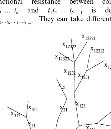
Using the example presented in Fig. 1, we can identify the structure of the model:
the depolarization at the trigger zone is
de-noted byXtz;
the potentials of the nearest (connected to the
trigger zone compartment) are denoted {Xi1}, i1=1, ...,P
1where
P1is the number of
these compartments; in Fig. 1, P1=3;
analogously, for the second level of the
com-partments connected to Xi1, the notation Xi1i2 is used,i2=1, ...,Pi1
2 . In Fig. 1,P 1 2=2,P
2 2=
1,P3 2
=2 and the number of higher branches is determined similarly (P113 =3,P123 =2 P213 =1,
and so on).
for a model with maximum number of
branch-ing levels B, the potentials at this level are denoted byXi1…iB; in Fig. 1, B=5.
The parameters (r, C) are indexed in the same way as the compartments and, analogously, the junctional resistance between compartments i1i2 ... ik and i1i2 ... ik+1 is denoted by
Ri1…ik, i1…ik+1. They can take different values for
different compartments. The following notation for constants is used throughout the rest of the paper ai1…ik=(ri1…ikCi1…ik)
−1, a
i1…ik, i1…ik+1= (Ri1…ik, i1…ik+1Ci1…ik)
−1 and the constant input
vector I0=(Itz, Ii1, Ii1i2, ..., Ii1i2…iB)
T. The
column vector of membrane potentials in all the compartments is denoted by X0 and a system of differential equations for its components can be written as follows.
(i) For a compartment that is neither a trigger zone nor the terminal one,
+d
dtXi1…ik+ai1…ikXi1…ik
=ai1…ik−1,i1…ik(Xi1…ik−1−Xi1…ik)
− %
Pi
1i2…ik k+1
j=1
ai1…ik,i1…ikj(Xi1…ik−Xi1…ikj)
+Ii1…ik (1)
(ii) The potential at the trigger zone is governed by the equation
+d
dtXtz+aXtz= %
P1
−j=1
aj(Xtz−Xj)+Itz (2)
where a(respectively aj) is the reciprocal value
of the trigger zone time constant (respectively junctional time constant between the trigger zone and connected compartments).
(iii) For the Kterminal compartments
+d
dtXi1i2…ib+ai1…ibXi1i2…ib
=ai1…ib−1, i1…ib(Xi1i2…ib−1−Xi1i2…ib)+Ii1i2…ib
b=b1, ..., bK (3)
This system of equations will be used for deter-mining the properties of the model.
2.2. Coding properties of the model
For long-lasting constant stimulation, a regular firing is achieved under the conditionSBXtz(),
where Xtz() is the asymptotic value of the
threshold. If tj and tj+1 are the times of the jth
and (j+1)th spikes in the activity of the model neuron, the aim is to derive a relationship between the length of the interspike interval (tj+1−tj) and the input I0. To solve this problem,
the system Eqs. (1) – (3) has to be investigated. Let X0 =(Xtz, X.d)T, where X.d is a Nd dimensional
vector of dendritic membrane potentials, simi-larly, letI0=(Itz, I.d)Tbe the decomposition of the
external inputs. Then, system Eqs. (1) – (3) takes the form dX0 /dt=MX0 +I0 with the following ini-order to find the time of the next spike, under the stationary firing, namely to find tj+1 such that
Xtz(tj+1) =S, the additional condition X.d(tj+
1)=X.d(tj) has to be imposed on this solution.
Let Qj(t)=eM(t−tj)
and consider the case in which an inverse matrix toMexists. Thus, we can write X0 (t)=[Qj(t)−1]M−1I0+Qj(t)X0 (t
j).
Tak-ing the decomposition of Qj(t) and M in
accor-dance with the trigger zone and dendrite, we have
M=
M1 M2vector, both withNdcomponents. A simple
calcu-lation gives the following two recalcu-lations:
[Q3j(tj+1)M2+Q4j(tj+1)M4−M4]X. dT(tj)
obtain the following Nd dimensional vector
equation:
which gives a closed relationship between inter-spike interval (tj+1−tj) and the external input.
We used a direct implementation of Eq. (4) as well as a numerical integration of system Eqs. (1) – (3). Both methods were compared and, in the examples presented later, they gave very similar results. Deriving the frequency of the spiking ac-tivity in the regular (stationary) regime from inter-spike intervals, for various external inputs, the rate coding properties of our model neuron can be deduced from this transfer function.
2.3. Examples
2.3.1. Example (a)
Previously, the relations between spiking fre-quency and different inputs were derived for a simple neuronal model composed of only two compartments with a single input at the dendrite, I0=(0, Id)T, (Bressloff and Taylor, 1994; La´nsky´
and Rodriguez, 1999a,b). This result can be di-rectly obtained from Eq. (4). To simplify, let us assume that both compartments have the same time constants. In such a case,
M=
−(a+ar) arar −(a+ar)
where ar and a are the inverse junctional and
transmembrane time constants. We denote
[arQ1
j(t
j+1)−(a+ar)Q2
j(t
j+1)−ar]
[−IdQ1
j(t
j+1)+Id+arS]=
[arQ2j(tj+1)−(a+ar)Q1j(tj+1)+(a+ar)]
[−IdQ2j(tj+1)−(a+ar)S]
This can be written in the form
Sa(a+2ar)[1−Q1
j(t j+1)]
+arId[Q2
j(t
j+1)−Q1
j(t
j+1)+1]
[Q2j(tj+1)+Q1j(tj+1)−1]=0.
This relationship can be obtained from the results presented by Bressloff and Taylor (1994), and is identical with formula (35) of La´nsky´ and Ro-driguez (1999a).
2.3.2. Example (b)
As a second example, let us take a model with four compartments: a trigger zone in series with a dendritic compartment that is connected to a couple of two parallel compartments, X0 =
(Xtz, X1, X11, X12). The system Eqs. (1) – (3) takes
the form
dXtz
dt = −(a+a1)Xtz+a1X1+Itz dX1
dt = −(a+a1,11+a1,12+a1)X1+a1,11X11
+a1,12X12+a1Xtz+I1
dX11
dt = −(a+a1,11)X11+a1,11X1+I11
dX12
dt = −(a+a1,12)X12+a1,12X1+I12
assuming aidentical for all compartments. Fig. 2 shows the frequencies of spike emission as ob-tained from Eq. (4) (points) and from numerical simulation of Eqs. (1) – (3) (lines) (using a Euler method with step dt=0.01 ms), for inputs applied only on the most distal compartments (dendrite 1 and dendrite 2 ), namelyItz=I1=0,I11,I12[−5,
20] mV/s. The threshold valueS=2 mV and the time constants have been chosen of the order of 10 ms. The values of parameters are a=0.1 ms−1, a
1,11=a1,12=1/16 ms−1, a1=0.9a1,11
Fig. 2. Transfer function for inputs on two distal compart-ments
ms−1, indicating a small variation of junctional
time constants along compartments.
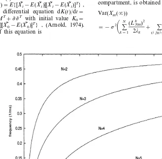
2.3.3. Example (c)
Let us consider a model with N compartments in series, X0 =(Xtz, X1, X11, X111, …, X1…1) ,
with an input applied to the most distal compart-ment whose depolarization is X1...1.
Fig. 3 shows how the transfer functions change in dependency on the number of compartments (the threshold S is kept fixed). The curves were obtained as solutions of Eq. (4) and verified by numerical integration. It follows from Fig. 3 that increasing, in this model, the number of compart-ments is accompanied by an increase of minimum signal intensity necessary to evoke a response.
3. The stochastic system
3.1. White noise perturbations and the filtering
process
subthreshold behavior, the deterministic system Eqs. (1) – (3) turns out to be aNd+1 dimensional
Ornstein – Uhlenbeck process given by the stochastic differential equation
dX0t=(MX0t+I00) dt+s˜ dWt X00=X(0)0
(5)
where I00 is constant input and Wt is a standard
Wiener process with amplitudes s˜=
(stz, si1, ..., si1i2…iB) specific for different com-partments. The mean behavior of the system of Eq. (5) is the same as the behavior of the deter-ministic system Eqs. (1) – (3). We will derive the second-order moments of X0t in order to
investi-gate the coding characteristics of the model neu-ron. Denoting K(t) the covariance matrix of the processX0t,K(t)=E{[X0t−E(X0t)][X0t−E(X0t)]
T} ,
it satisfies the differential equation dK(t)/dt=
MK(t)+K(t)MT+s˜s˜T with initial value K
0=
E{[X00−E(X00)][X00−E(X00)]T} , (Arnold, 1974).
The solution of this equation is
K(t)=eMt
K0e
Mt
+
&
t
0
eM(t−s)s
˜s˜TeM(t−s)ds (6)
As an example of application of this formula, we consider the last model of Section 2.3.3 (N com-partments in series). For the elements of K(t) Kij(t)=[Q(t)K0Q(t)]ij
+s2
&
t
0
QiN(t−s)QNj(t−s) ds (7)
where Q(t)=ke
lkt
j"k[(M−lj)/(lk−lj)] and
li, i=1, …, N are the (negative) eigenvalues of
the (symmetric) N×N matrix M. Integration in Eq. (7) can be performed, and the limiting value ofKmm(t) ast , which is the asymptotic value
of the variance of the depolarization of the mth compartment, is obtained as:
Var(Xm())
= −s2
%N k=1
(LNm k )2
2lk
+ %
(i j)(i"j)
LNm
i L Nm j
(li+lj)
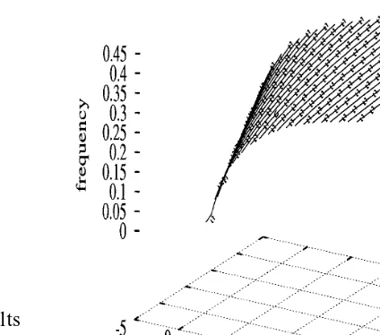
(8)Fig. 3. Transfer function for a model withNcompartments in series. The reciprocals of time constantsajbetween compartments
Fig. 4. Trajectories of depolarizations in the stochastic model. The parameters ares11=5.0 mV ms,a=0.1 ms−1, ar=1/16 ms−1,I
d= 10 mV ms−1. where LNm
k are elements of
Lk
=j"k[(M−lj)/
(lk−lj)]. The asymptotic covariances can be
ob-tained in the same way. It follows from Fig. 4, in which the behavior of the depolarization in this model is illustrated (N=3, X0 =(Xtz, X1, X11)
T
ands˜=(0, 0, s11)T), that a decrease of stochastic
fluctuations occurs from the dendritic part to the trigger zone. This decrease of variability along three compartments can be analyzed by using Eq. (8). Of course, this effect occurs also for the two-compartment model for which the formulas are simpler and thus presented here. In that case,
M=
−(a+ar) arar −(a+ar)
with eigenvalues l1= −a, l2= −a−2ar, where
a and ar correspond to the reciprocals of time constants for transmembrane current and for cur-rent between the trigger zone and the other (den-dritic) compartment. We have
Var(Xtz())= −
s2
4
1 2l1+ 1
2l2
− 2
(l1+l2)
and
Var(X1())= −
s2
4
1 2l1+ 1
2l2
+ 2
(l1+l2)
The decreasing variability from the dendrite to the trigger zone follows clearly from these formulas; these results were obtained by another method by La´nsky´ and Rodriguez (1999a).3.2. Poissonian inputs and mean transfer functions
The continuous trajectories of the membrane depolarization are the main characteristic of the already described multicompartmental model. The reason is that the model does not consider the soma of the neuron as its specific part, where the contributions to the membrane depolarization are not so frequent (not so many synaptic endings are located there as on the dendrite) but of substan-tial size. While the input at the dendrite causes small changes of the membrane potential, and thus the system is well characterized by the white noise, it would be natural to expect that the incoming signal located at the soma and near the soma has discontinuous effect on the depolariza-tion. This leads to the investigation of a model neuron where the stochastic part also includes Poissonian inputs. Let us consider the following system: stochastic process with components of the form
zj=sjWj+ajNj
+
+bjNj
−. Here, s
j is the
ampli-tude of the white noise part withWjas Brownian
motion acting on the jth compartment, and Nj
+
(resp. Nj
−) are (independent) Poisson processes
with intensities l+j (resp. l
j
−) that drive synapses
on this compartment for which excitatory and inhibitory postsynaptic potentials have their am-plitudesaj(resp.bj). For this neuronal model, one
can derive a relation between estimate of the mean interspike interval and the constant input I00. This can be done by using Eq. (4), with I0
identified as I0=I00+K0 , where Kj=ajl+j +bjl−j .
The transfer functions deduced in this way were compared with those obtained by simulation of system of Eq. (9). Here, only a simple example is presented, in which the neuron is composed of three compartments in series,X0 =(Xtz, X1, X11)
T,
with constant plus white noise input acting onX11
and Poissonian impulses impinging on X1. Using
the same notation for the parameters as before, the stochastic system of Eq. (9) is
dX11=[−(a+a1,11)X11+a1,11X1+I11] dt
+s11 dW
dX1=[−(a+a1,11+a1)X1+a1,11X11+a1Xtz] dt
+a1 dN+1 +b1 dN−1
dXtz=[−(a+a1)Xtz+a1X1] dt
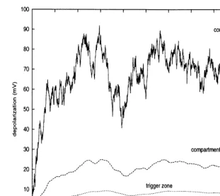
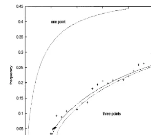
The input – output functions for this system are plotted in Fig. 5, where a comparison with the single-compartment model (with the same time constant a−1
) is also shown (curve on the left). The dashed curve on the right corresponds to the deterministic case (s11=a1=b1=0). The dashed
curve in the middle corresponds to the mean frequencies of the stochastic system as obtained from Eq. (4). Finally, the crosses were obtained from simulated mean interspike intervals.
A numerical procedure of Euler type was used in order to solve this set of stochastic equations. For the Brownian part, in the first equation, at each time step of length Dt, a random variable z=s11Dtuwas generated whereu is a Gaussian
variable of zero mean and variance equal to one. In the second equation, a set of exponentially distributed random time intervals between jump instants, with parameters l1
+
(resp. l1
−
), was gen-erated. The process N1
+
(t) (resp.N1
−
(t)) was built with jumps of amplitude unity at the jump in-stants. At each time step of length Dt, at time t, the new value of X1, for the Poissonian part, was
achieved by adding a1[N1
Fig. 5. Transfer functions for stochastic models with Poissonian and white noise stimulations. The parameters are a1=5 mV,
b1= −2 mV,l+1=0.1 ms−1,l−1=1/12 ms−1,s11=2 mV/ms,S=5 mV,a=0.1 ms−1,a1=a1,11=1/16 ms−1.
possibly complex dendritic structure, can still be analyzed using classical vectorial deterministic and stochastic calculus.
It was generally considered that the coding range of the one-point integrate-and-fire model was too narrow and the threshold input intensity for spike emission was too low as compared with those experimentally observed. The introduction of spa-tial structure in the model removes, at least partly, these drawbacks. When noise is considered in the input and acts on the dendritic part, a filtering occurs naturally from dendrites to the zone of spike generation. This makes the neuron more robust against fluctuating perturbations. Thus, the multi-compartmental integrate-and-fire models, as com-pared with more complex and more realistic conductanced-based models that can be generally investigated only numerically, may be viewed as convenient prototypes for the analytical study of spiking neurons.
Acknowledgements
This work was supported by Academy of Sci-ences of the Czech Republic Grant No. A7011712/
1997 and by GIS ‘Sciences de le Cognition’ Grant CNA 10. The authors thank Severine Tramoni for help in the implementation of numerical methods.
References
Arnold, L., 1974. Stochastic Differential Equations: Theory and Applications. Wiley, New York.
Bressloff, P.C., 1995. Dynamics of compartmental model inte-grate-and-fire neuron with somatic potential reset. Physica D 80, 399 – 412.
Bressloff, P.C., Taylor, J.G., 1994. Dynamics of compartmen-tal model neurons. Neural Networks 7, 1153 – 1165. Bulsara, A.R., Lowen, S.B., Rees, C.D., 1994. Cooperative
Bulsara, A.R., Elston, T.C., Doering, C.R., Lowen, S.B., Lindenberg, K., 1996. Cooperative behavior in periodically driven noisy integrate-and-fire models of neuronal dynam-ics. Phys. Rev. E 53, 3958 – 3969.
DeSchutter, E., 1989. Computer software for development and simulation of compartmental models of neurons. Comp. Biol. Med. 19, 71 – 81.
Edwards, D.H., Mulloney, B., 1984. Compartmental models of electrotonic structure and synaptic integration in an identified neuron. J. Physiol. 348, 89 – 113.
La´nsky´, P., Rodriguez, R., 1999a. Two-compartment stochas-tic model of a neuron. Physica D 132, 267 – 286. La´nsky´, P., Rodriguez, R., 1999b. The spatial properties of a
model neuron increase its coding range. Biol. Cybern. 81, 161 – 167.
La´nsky´, P., Rospars, J.P., 1995. Ornstein – Uhlenbeck model neuron revisited. Biol. Cybern. 72, 397 – 406.
Perkel, D.H., Mulloney, B., 1978. Electrotonic properties of neurons: steady-state compartmental model. J. Neurophys-iol. 41, 621 – 639.
Perkel, D.H., Mulloney, B., Budelli, R.W., 1981. Quantitative
methods for predicting neuronal behavior. Neuroscience 6, 823 – 837.
Plesser, H.E., Tanaka, S., 1998. Stochastic resonance in a model neuron with reset. Phys. Lett. A 225, 228 – 234. Rospars, J.P., La´nsky´, P., 1993. Stochastic model neuron
without resetting of dendritic potential. Application to the olfactory system. Biol. Cybern. 69, 283 – 294.
Segev, I., 1992. Single neuron models: oversimple, complex and reduced. TINS 15, 414 – 421.
Segev, I., Fleshman, J.W., Burke, R.E., 1989. Compartmental models of complex neurons. In: Koch, C., Segev, I. (Eds.), Methods in Neuronal Modeling. MIT Press, Cambridge. Shimokawa, T., Pakdaman, K., Sato, S., 1999. Time-scale
matching in the response of a leaky integrate-and-fire neuron model to periodic stimulus with additive noise. Phys. Rev. E 59, 3427 – 3443.
Tuckwell, H.C., Rodriguez, R., 1998. Analytical and simula-tion results for stochastic Fitzhugh – Nagumo neurons and neural networks. J. Comp. Neurosci. 5, 91 – 113. Tuckwell, H.C., 1988. Introduction to Theoretical
Neurobiol-ogy. Cambridge University Press, Cambridge.