ANALYSIS
The effects of ageing and an environmental trust fund in an
overlapping generations model on carbon emission
reductions
Reyer Gerlagh
a,*, B.C.C. van der Zwaan
a,baVrije Uni6ersieit Amsterdam,Institute for En6ironmental Studies,De Boelelaan1115,1081HV,Amsterdam,The Netherlands bStanford Uni6ersity,Center for International Security and Cooperation,Encina Hall,Stanford,CA94305-6165,USA
Received 3 January 2000; received in revised form 30 May 2000; accepted 25 July 2000
Abstract
Most currently employed Integrated Assessment Models for climate change are of a dynastic nature. They employ the Ramsey rule linking the interest rate, economic growth, and the rate of pure time preference. This paper argues that, although a dynastic framework might be convenient for economic analysis, it is restrictive and can be misleading. Overlapping Generations models, which do not employ the Ramsey rule, are more flexible and may give results different from those derived from dynastic models. With the Integrated Assessment Model ALICE 2.0, it is shown how various assumptions on demographic change and public institutions can affect the interest rate, thereby influencing the efficient greenhouse gas emission reductions. It is concluded that dynastic Integrated Assessment Models are in many respects inappropriate for providing policy makers with quantitative figures about the costs of carbon dioxide emissions and their desirable reduction levels. © 2001 Elsevier Science B.V. All rights reserved.
Keywords:Resource conservation; Discounting; OLG models; IAMs; Ageing; Trust funds
JEL classification:C68; J19; H43; Q28; Q48
www.elsevier.com/locate/ecolecon
1. Introduction
Recently, environmental and resource economists have increasingly been considering
large scales of time. Problems such as a potential climate change, the exhaustion of natural re-sources, or the safe disposition of long-lived ra-dioactive nuclear waste, compel current generations to take into account to a high degree what the results are of their actions in the far future. In the context of a large time horizon, the discount rate determines the outcome of economic * Corresponding author. +31-20-4449555; fax: +
31-20-4449553.
E-mail addresses: [email protected] (R. Gerlagh),
[email protected] (B.C.C. van der Zwaan).
analysis to a larger extent than in research with respect to short-term questions.
This paper draws attention of the increased relevance of accounting properly for the discount rate in economic modelling. In particular, this will be done with respect to the phenomenon of global warming, which since the summits of Rio and Kyoto has become high on the agendas of both politicians and scientists. Since a potential climate change caused by anthropogenic greenhouse gas (GHG) emissions has been recognised as a major environmental problem, a number of so-called Integrated Assessment Models (IAMs) have been developed to advise policy makers on the costs of current GHG emissions and on the desirable GHG emission reduction levels. From these IAMs, one can derive strategies with respect to the efficient levels of greenhouse gas concentrations in the atmosphere, and estimate the expected global ef-fects of a ‘business as usual’ carbon dioxide emis-sion pattern. Among the score of IAMs developed since the beginning of the 1990s, some of the more well known are CETA (Peck and Teisberg, 1992), DICE (Nordhaus, 1994), MERGE (Manne and Richels, 1995 ), MERGE-II (Manne et al., 1995) and RICE (Nordhaus and Yang, 1996).
Most IAMs presently used are of a dynastic type.1 They assume, some more and others less
explicitly, a central planner maximising a welfare measure which aggregates utilities over different generations. The allocation of consumer goods and environmental resources is calculated from the rules for welfare distribution over these genera-tions. Alternatively, in a so-called overlapping generations (OLG) framework, the dynamic alloca-tion is primarily determined by the distribualloca-tion of property rights over generations.2 The analysis of
many dynastic models has led to intensive debate on the kind of welfare functions to be used (see, for example, Azar and Sterner, 1996). In this paper, it is argued that the dynastic mechanism of welfare distribution exhibits characteristics that are unreal-istic, sometimes even misleading. Its prevalent use in IAMs has led to unnecessary controversies between researchers advocating efficient resource use, on the one hand, and those who advocate resource protection, on the other hand.
The dynastic IAMs commonly use a constant Rate of Pure Time Preference (RPTP) to discount future welfare levels before aggregation into a net present welfare measure.3
A low RPTP implies that future benefits and costs are valued relatively highly, whereas the use of a high RPTP means that relatively little value is attached to future benefits and costs. The discount rate considerably affects the calculation of the emission costs and the corresponding efficient carbon dioxide emission levels. Because of the importance of the role played by the discount factor in economic modelling, the precise value to be taken is subject of invariable controversy.
Some economists suggest that historic data on interest rates can be used to calibrate the level of the RPTP used in IAMs, while these in turn determine the efficient environmental resource use (Nordhaus, 1994, Chapter 6). In their opinion, time preference should be based on past evolution of the human use of resources. In other words, they assume that historic data determine which environ-mental resource use is economically feasible. Others strongly oppose this so-called
‘descrip-3For a more general welfare aggregation, which employs a so-called aggregator function that has no constant RPTP, see Koopmans (1960) and Koopmans et al. (1964). The distinction between a constant and variable RPTP is not without impor-tance. Lucas and Stokey (1984), as well as Epstein (1987), point out that if one presumes a constant RPTP, the steady states of the economy constitute a continuum. They state that this is an unrealistic characteristic of long-term economic behaviour. It is a direct result of the assumption of time-addi-tivity, which in their opinion is a mere artefact of economic modelling.
1Dynastic models are also referred to as ILA (infinitely lived agent) or Ramsey models. We favour the term ‘dynastic’ since it has a natural connotation to the empathy between generations that form a dynasty. It includes OLG models with empathy, since they have the same analytical properties as pure Ramsey models (see e.g. Barro, 1974).
2OLG models exist with dynastic properties, as mentioned in footnote 1. Generally, however, OLG models do not assume interpersonal comparability (see Roberts, 1980, for a discus-sion in relation to public choice theory) and have rather different dynamic properties (Geanakoplos and Polemar-chakis, 1991; Kehoe, 1991).
-tive’ view, which normally leads to using relatively high values of the discount rate, and argue for a ‘prescriptive’ approach. Here, one uses a low dis-count rate since future generations should not be discriminated against by lower welfare weights (see, for example, Broome, 1992). The rationale behind this is that if discounting is too high, it is normally considered economically unfeasible to sustain a high quality environment.
In practice, it proves difficult to bridge the gap between the ‘descriptors’ and ‘prescriptors’. In this paper, it is argued that part of the disagree-ment between their opposing views is due to the fact that both use a dynastic framework. Such a dynastic approach gives a convenient simplifica-tion of the dynamic competitive equilibrium, but it treats discounting with insufficient reality. In a dynastic model with constant RPTP, the interest rate is rigidly linked to economic growth via the Ramsey rule, r:r+gg, where r is the interest rate, r is the RPTP, 1/g is the intertemporal elasticity of substitution, and g is consumption growth (see e.g. Cline, 1992). Using an OLG-model allows for a more flexible relation between interest rate and economic growth since there is no central planner and, consequently, there is no planner’s rate of pure time preference. Various factors can result in changes in the interest rate over time, such as local or global demographic changes,4or a modification of the regime designed
to preclude an over-exploitation of the environment.
These possible, or even likely, exogenous and endogenous changes render the extrapolation of the overall trend of historic interest rates to the future unjustified, as well as the rigid dynastic assumption inappropriate. Therefore, we suggest not employing a rigid discounting relation as is common practise in dynastic models. To show that the more flexible OLG approach is feasible in
the IAM context, we present ALICE 2.0, an Integrated Assessment Model with Overlapping Generations (OLG-IAM) applied to the issue of climate change. The model extends the usual IAMs — including the OLG-IAMs by Stephan et al. (1997), Howarth (1998), and Manne (1999) — in three respects: it contains a demographic transi-tion, it specifies environmental damages as a loss of an environmental amenity associated with an environmental resource, and it specifies a transfer mechanism that distributes the value of this re-source to consumers. Although all three elements have been studied — to some extent at least — before, see e.g. Auerbach et al. (1989), Krautkrae-mer (1985), and Howarth and Norgaard (1992), respectively, the novelty of our analysis lies in the fact that we introduce these elements in one con-cise OLG-IAM with climate change. Vis-a`-vis the intergenerational distribution of property rights over environmental resources, this paper follows the recent theoretical literature that analyses re-source use in the context of OLG models (Howarth and Norgaard, 1992; Gerlagh and Keyzer (forthcoming). Yet, distributing ‘climate endowments’ over generations is to some extent premature, given the small number of environ-mental goods over which property rights have been established so far, and given the slowness with which the set of such goods is currently expanded. Practicable policy suggestions require the use of a richer OLG model (for a more elaborate discussion, see Farmer and Randall, 1997). Nonetheless, the numerical results demon-strate that future interest rates can readily de-crease below the levels predicted by the descriptive approach in dynastic models.
The paper proceeds as follows. Section 2 de-scribes ALICE 2.0, designed for the analysis of greenhouse gas policies on a world economy level. The model elaborates on ALICE 1.2, which is extensively described and analysed in Gerlagh and van der Zwaan (forthcoming). Section 3 specifies four scenarios with different assumptions regard-ing future demographic change and regardregard-ing the distribution of ‘climate endowments’. Section 4 compares the numerical outcomes of the scenar-ios. Finally, Section 5 draws conclusions.
2. Model specification for ALICE 2.05
This section focuses on a description of popula-tion dynamics, of consumer and producer be-haviour, of markets, and of the savings balances. The model distinguishes discrete time steps,
tT={1, …,}, representing periods of 20 years each. To solve the model numerically, it is trun-cated after a periodT.
2.1. Population
The first period corresponds to the interval 2000 – 2020. In every interval a new generation is born. The model only describes the adult part of the life-cycle, i.e. from the age of 20 onwards. This implies that a two-period life represents an individual who reaches the age of 60, and a three-period life an individual reaching the age of 80. Consumption of children, in the age between 0 and 20, is accounted for by consumption of their parents. A generation is called young when its members have an age between 20 and 40; middle-aged are those individuals between 40 and 60, and old is the generation with members between 60 and 80.
Each generation is denoted by the date t on which it starts consumption; it then enters the model. The generation denoted t is born at time
t−1.6 Generations are of different size, denoted
bynt. The life-cycle lengths of generations are not
identical. A demographic change is specified to represent increasing life expectancy, modelled as a transition from a life-cycle of two periods to one of three periods. This transition is supposed to take place entirely during the 21st century, that is, during the first five intervals considered in the model. In the first interval, only a young and
middle-aged cohort coexist, without the presence of an old-aged generation. The middle-aged in the first interval die at the end of that interval. Twenty percent of the young in the first interval, i.e. the middle-aged in the second interval, live for a third period. Hence, in the third interval there is a small group of old consumers. Of the young generation in the second interval, i.e. the middle-aged of the third interval, forty percent live three periods, while the others live only for two periods. Life expectancy continues to increase linearly un-til all members of the generation that is young in the 2080 – 2100 interval live through a life-cycle of three periods. The life expectancy transition is then completed.
Let nt
i denote the size of generation i in interval
t, so that nt
idenotes the size of generationiwhen
it starts consumption. We assume that no member of a generation dies before the start of the second consumption period of its life: ntt+1=nt
t=nt, for
all generations t. As noted, the increase in life expectancy implies that the number of people living the full three periods increases linearly:
n31=0.2n21,n42=0.4n32, and so forth, untiln75=n65.
The time evolution of the size of a generation is defined recursively according to a logistic growth curve:
nt+1
=(an −(an
−1)(nt
/n¯))nt, (1)
where n¯ is the maximal size of a cohort, and an
the growth factor if nt is small with respect to n¯.
The population sequence nt depends on n0, the
size of the first generation that enters the model, and on the variables an, andn¯ via Eq. (1). These
parameters are calibrated such that the series approximates World Bank (1994) data on global population. See also Gerlagh and van der Zwaan (1999) for a slightly more detailed description of population growth. The results are shown in Table 1. The table also shows the modelled in-crease in life expectancy used in ALICE 2.0, which reasonably captures the main characteris-tics of the World Bank forecasts on life expec-tancy. Anticipating an alternative scenario analysis in Section 3 that abstracts from ageing, we also calibrated parameters for the case in which ntt+2 is set to zero for all t.
5ALICE is the acronym for Applied Long-term Integrated Competitive Equilibrium model.
Table 1
Population and life expectancy in ALICE 2.0
2100
1960 1980 2000 2020 2040 2060 2080 2200
11.0
Population WBa n.a. n.a. 6.1 7.7 9.0 9.9 10.6 n.a.
11.1 Population ALICE 2.0 (ageing)b n.a. n.a. 6.1 7.7 9.0 10.0 10.7 11.1
11.0 Population ALICE 2.0 (no ageing)b n.a. n.a. 6.1 7.6 9.0 10.0 10.6 11.3
n.a. Life expectancy at birth WBa n.a. 63.5 67.4 71.2 74.7 77.9 80.3 82.6
80.0 Life expectancy at birth ALICE 2.0c 60.0 64.0 68.0 72.0 76.0 80.0 80.0 80.0
aPopulation is in billion people and life expectancy in years, calculated from World Bank data (WB, 1994).
bThe population at the beginning of periodtis taken to be the average population of periodst−1 andt. The population in period
tincludes the children who enter the model one period later. Both population sequences, with and without ageing, are calibrated to the WB data.
cWith ageing.
3. Consumers
Generations maximise their lifetime utility
u(ct,bt), derived from rival consumption of the
consumer good during the life-cycle,ct =(ct
t
,ct+1 t
,
ctt+2), and non-rival consumption of the resource
amenity, for convenience referred to as ‘environ-mental services’,bt
=(bt,bt+1,bt+2). We omit the
superscript t in the consumption of the resource amenity to stress that the amenity consumption is the same for all generations alive at period t. By this definition of utility, an extension is made with respect to conventional IAMs, since the latter treat climate change damages as if they would constitute merely a decrease of man-made con-sumer goods. We think that a large part of the damages caused by global warming can be under-stood as a decrease in the quality and quantity of environmental functions, much more than as a reduction in the flow of man-made goods. Indeed, the IPCC (1996b, Section 1.3.2) recognises that a decrease in biodiversity may be one of the major consequences of climate change. Our explicit spe-cification of a resource amenity provides a means to incorporate this insight into a competitive equi-librium framework. In order to allow for covering a more complete range of climate change effects, we would need to model both amenity and pro-ductivity effects. An extension of our model with respect to these effects is one of the potential fields of future research.
The consumption behaviour of generations from which not all members live three periods is
based on some further assumptions. For any member of a generation, until the beginning of the third period, only the probability of living three periods is known. At the beginning of the third period, any member is either alive or not. Each member is supposed to maximise expected life-time utility. There are no non-intended bequests to future generations resulting from the uncer-tainty in life-time (Hurd, 1989), because there is an intra-generational life insurance company to which all members of a generation pay their sav-ings in the second period of life. The insurance company repays the savings to the living members of the generation in the third period. Under this condition, there is no need to explicitly describe the actions of the insurance company and of separate consumers; one representative consumer who maximises aggregate utility, subject to one budget constraint, can describe the generation.7
The utility functionu(·) employed is a nested CES function of form:
u(ci,bi) =
%i+2
t=i
(s)t−in t i((c
t
i)1/(1+n)(b t)
n/(1+n))(r−1)/r
n
r/(r−1),
(2)
where r=0.67 is the intertemporal elasticity of substitution, s=1 is the consumers’ time
ence factor,8and
n=0.1 is the constant share of the expenditures on the resource amenity relative to the man-made consumer good:
i are the so-called Lindahl prices for
generationiin periodtfor non-rival consumption of the resource amenity, relative to the price of the man-made consumer good.
The first generationi=0 maximises utility sub-ject to its budget constraint:
max{u(c0
where prices are normalised so that the consumer good has price unity, bit is the price depreciation
factor from periodito periodt(whenever conve-nient, we also write bt for btt+
1
), wt denotes the
price of labour,lt i
denotes the labour endowment, c1is the price of the man-made capital stockk1in
the first period owned by the first generation, and
Ht
i is the income which generation
i receives in periodtas its share in the value of the environmen-tal resource. For generation i, the first order condition for the first choice variableciis given by:
(ui(·)/(ci=li(1,b i i+1,b
i
i+2). (6)
for some scalarli\0. Non-rivalry of the demand
for the resource amenity implies that consumers should agree on the provision of the amenity level and jointly finance them. Thus, Lindahl prices8ti
should add up to the production price ptb:
pt
and the first order condition for the choice variable
bi should satisfy:
(ui(·)/(bi=li(8
the budget in Eq. (5) holds.
3.1. Producers
ALICE 2.0 includes a simple production sector for a man-made consumer good yt, consisting of
one private firm. It uses labour units lt, emission
units et, and a man-made capital stock kt as
production factors. The capital stock is itself pro-duced by this production sector. We therefore assume that the capital stock is made up of the consumer good, and that it has to be replaced after use in one period. The production structure is based on a nested function, in which the intermediate goodytmis made of a Cobb – Douglas composite of
capital and labour:
ytm=Atktalt1−a, (9)
where At is a productivity coefficient. 9
The com-posite good yt
m
is used, together with emission units, in a quadratic production function:
yi+kt+1=yt m
+12(h/zt)et(2zt−et/yt
m), (10)
where h is the maximal CO2 tax at which net
emissions become zero, and zt is the maximum
emission intensity when no carbon taxes are im-posed. This becomes clear from the first order condition for emissions:
pte]h(1−et/ztytm)Þet]0, (11)
wherepteis the price of emission units in periodt,
and the complementarity sign ‘Þ’ denotes that the left-hand inequality is binding (i.e. becomes an equality) if emissions are positive. The parameters h and zt are chosen such that the efficient
emis-8The intertemporal elasticity of substitution, r, and time preference,s, are based on estimates in the literature (Davies, 1981; Auerbach et al., 1989; Hurd, 1989). Note that in an OLG model, there is no a priori reason to have a strictly positive time preference rate, represented throughsB1. Re-placings=1 by a valuesB1 would result in higher interest rates in all scenarios, though qualitatively, results would not change. For a detailed calibration analysis, see Gerlagh (1998b, Section 4.2.3).
sion levels decrease by 1 percent for every 4 US$/tC price increase of emission units,10 and
that the maximum emission levels follow the IS92a scenario (IPCC, 1992). The IS92a bench-mark scenario assumes an autonomous decrease in the emission intensity zt , partly based on an
autonomous increase in energy efficiency (AIEE) and an autonomous expansion of backstop technologies.
Because of constant returns to scale, the value of inputs equals the value of outputs:
yi+kt+1=wili+ctkt+pt e
et, (12)
wherect is the price for capital in periodt. Since
capital is produced in the previous period, we have:
ct+1=1/bt, (13)
for t=1, …,. After substitution of the value Eq. (12), we have the following first order condi-tions for labour and capital:
wtlt=(1−a)(yt+kt+1−pt ee
t), (14)
and
ctkt=a(yt+kt+1−pteet). (15)
3.2. Climate change
As noted above, ALICE 2.0 extends the exist-ing IAMs by specifyexist-ing an explicit resource amenity, following Krautkraemer (1985). In terms of the model, the biogeochemical system produces emission unitset, and environmental servicesbt. It
is a renewable resource that, however, deteriorates because of emissions, and this is the core of the problem (Clark, 1997). This is in accordance with the environmental concerns underlying the issue of climate change.
We will now describe how this resource amenity relates to greenhouse gas emissions. As the emis-sions of CO2account for the main anthropogenic
contribution to the greenhouse effect, we focus on
the carbon cycle and its relation to climate change. ALICE 2.0 follows CETA (Peck and Teisberg, 1992), linking emissions to concentra-tions, concentrations to temperatures, and tem-peratures to damages. We use the ‘linear box’ model in which one distinguishes between five separate spheres, each having different properties with respect to carbon dioxide absorption (Maier-Reimer and Hasselmann, 1987). It is assumed that the CO2emitted is distributed over the five boxes
in amounts corresponding to shares ai(i=1,…,5)
of total emissions. Within each box, the CO2
concentration exponentially adjusts to its natural level at an annual adjustment rate 1/ti. Let st i
denote the accumulated anthropogenic emissions in box i at the beginning of period t. We then have:
st=1
i =e−N/tis
t i+a
iet, (16)
where Siai=1 and N is the period length in the
discrete time model.The accumulation of GHGs causes an increase of the equilibrium global mean temperature. For CO2, the temperature increase is
expected to be of approximate logarithmic nature,
Tt eq
=T( 2
log
1+%i
st i
/s¯
, (17)where Tt
eq is the long-term equilibrium
tempera-ture for given concentrations Sist i, and
T( is the benchmark equilibrium temperature associated with a doubling of total accumulated anthropo-genic GHGs in the atmosphere compared with the ‘natural’ level s¯ (see IPCC, 1992).
The earth surface and atmosphere have a cer-tain warmth capacity. Therefore, the temperature, denoted by Tt, slowly adjusts to the long-term
equilibrium level:
Tt+1=e−NoTt+(1−e−No)Tt+1 eq
, (18)
where o is the annual adjustment rate.
However, when calculating impacts of climate change, the scientific understanding is grossly in-sufficient to warrant even something like a ‘best guess’ (IPCC, 1996a, Section 6.2.13). In general, it is assumed that damages caused by climate change will outweigh its benefits. The lack of knowledge is unmistakably revealed by the sensi-tivity analyses carried out with a variety of differ-10This value is an average of the numbers found in the
ent damage functions (cf. Tol, 1995). These damage functions are supposed to provide a re-duced form of the many complex damages asso-ciated with climate change, such as the loss of coastal zones due to sea level rise, the loss of biodiversity, the spread of vector-borne diseases, and the occurrence of extreme climate events. Most IAMs subtract damages from production or consumption, or directly from utility. ALICE 2.0 differs from these models and defines a non-rival good labelled ‘environmental services’, which level is given by:
bt+1=e
−Nd
bt+(1−e
−Nd
)(1−f(Tt+1)), (19)
where Tt is the global mean surface temperature
relative to the pre-industrial level, d is the an-nual adjustment rate, and f(·) is the reduced form function that describes long-term losses of environmental services which we take to be in-creasing on its positive domain, and for which
f(0)=0; see (Tol, 1995) for various functions.11
For ALICE 2.0, f(·) is taken to be quadratic, and f(Tt+1)=1 for Tt+1 a 6°C temperature
in-crease. Hence, for a 3°C temperature increase (the usual benchmark case for 2100), the long-term resource amenity decreases by 25 percent. By taking the value share of the resource amenity as 10 percent (n=0.1 in Eq. (2)), this amounts to a welfare loss equivalent of a 3 per-cent decrease of GDP.
These assumptions on climate change damages imply that, over the next century, welfare in-crease through economic growth will more than compensate any level of climate change dam-ages. Concerns for decreasing welfare levels are thus unwarranted. We accept these benchmark values, not because we adhere to this optimistic view, but because we want two areas of debate well separated. On the one hand, a debate on the correct estimation of present costs and fu-ture benefits of climate change regulations (to which we do not pretend to contribute), and on the other hand the question as to the effect on
actual resource use of including demography and using various distributional rules. We will abstain from presenting welfare levels which we do not think to be reliable, but only show graphs that are directly related to the resource use, and refer to an early stabilisation of climate change as resource conservation.
3.3. Markets
We have the commodity balance for labour,
lt=lt
and for the consumer good,
ct
The regulatory mechanism for controlling re-source extraction and distributing income from the natural resource, as well as the correspond-ing regulations, are specified in Section 3. The Lindahl equilibrium represents an economy gov-erned by a mixture of competitive markets and policies to achieve collective action. Since the summation of budgets of all generations has to balance, the sum of the resource income shares should equal the total value of the resource, that is:
t is the price deflator for period t
rela-tive to period 1, where the income claim is dif-ferentiated by date of accrual using the super-and subscripts as Ht=H
this allows defining the period-specific claim as
Ht=Htt+ +Htt−1+Htt−2. Notice that
genera-tion t=0 only has a claim H10 to the resource.
3.4. Sa6ings balances
For the coming analysis, it is convenient to distinguish between the value of the environ-mental resource at any point in time,
Vt= %
and the value of total assets to be reserved in any period t for meeting future claims,
11If a decrease in the amenity b
t persists, this could be incorporated (e.g. in a possible next version of our model) by takingbt+1to constitute the minimum ofbtand the RHS of
Ft= %
These relations can be written recursively as
Vt=pt
To implement the intergenerational distribution of claims Hti, we introduce a trust fund that
reserves the value of total assets. In particular, income from emission taxes is not directly dis-tributed among the generations alive (the pol-luters), but is attributed to the trust fund for meeting future claimsFt, so that every generation
in every period is paid its share Ht
i, according to
Eq. (26). Initially, the trust fund assets equal total resource income shares, which should sum to the total value of the resource, that is:
F1=V1. (27)
We are now in a position to specify the savings-capital balance, which has a central role in the scenario analysis. Let Stt+1 and Stt+2 be the
sav-ings of generation t at the beginning of period
t+1 andt+2, respectively. These are defined by the expenditure budgets when young,
btSt+1
The life-cycle budget constraint Eq. (5) ensures that savings are exhausted when old:
0=St+2
The capital-savings balance equals total sav-ings, which consists of private savings plus the assets held by the trust fund, with the value of capital, which consists of man-made capital and the resource value:
Stt−1+Stt−2+Ft=ctkt+Vt. (31)
The equation explicitly shows the trust fund’s wealth transfer to future generations through sav-ingsFt that are additional to private savingsSt
i. A
more extensive description of the set up and working of a trust fund is given in Gerlagh and Keyzer (forthcoming). Validity of the savings-cap-ital equation fort=2 is ensured by summation of Eqs. (4), (27) and (28), subtracting Eqs. (12) and (20) multiplied by wages w1, (Eq. (21)), (Eq. (7))
multiplied by the amenity level b1, and (Eq. (26)).
After using (Eq. (13)) for substitution, we have:
b1(S2 1
+F2)=b1(c2k2+V2), (32)
which is the second period savings-capital balance multiplied by the price factor b1.
12 For
t= 3, …,, validity follows from forward induction.
To complete the model specification, we define equilibrium:
Definition 1. A competitive equilibrium of model Eqs. (1) – (31) is an intertemporal allocation sup-ported by prices wt,pte,ptb,8tt−2,8tt−1,8tt,ct,bt,
fort=1, …,, that satisfies the production iden-tities Eqs. (9) and (10), the environmental identi-ties Eqs. (16) – (19), the first order conditions Eqs. (6) – (8), (11), (13) – (15), the commodity balances Eqs. (20) and (21), the savings identities Eqs. (28) and (29), and the savings-capital balance Eq. (31), for a given environmental regulatory policy that satisfies Eqs. (25) – (27).
3.5. Scenario specification
ALICE 2.0 is calibrated to replicate the so-called Business as Usual IS92a-scenario (IPCC, 1992) for the case that climate change is not internalised in the economy. This benchmark sce-nario is not displayed in this paper. Four scenar-ios are specified to show how the demographic change and the intergenerational distribution of property rights over the environmental resource affect efficient climate change policies vis-a`-vis emission reductions. The scenarios are sum-marised in Table 2. The first scenario, labelled I,
Table 2
Scenario specification
No ageing Ageing included
‘Victims pay’ Environmental resource Scenario I endowed to first generation:
Grandfathering — No ageing Scenario II Grandfathering — Ageing Grandfathering
‘Polluters pay’ Environmental resource Scenario III Scenario IV shared with future generations:
Trust fund Trust fund — No ageing Trust fund — Ageing
assumes that the environmental resource is given, or ‘grandfathered’, to the first generation. This scenario abstracts from any increase in life expec-tancy. The second scenario, labelled II, includes the above-described demographic change, in addi-tion to the grandfathering of the environmental resource to the first generation. Since grandfather-ing implies that future generations will have to pay if they want to enjoy a clean environment, scenarios I and II may collectively be denomi-nated ‘Victims Pay’. The third scenario, labelled III, assumes that the property rights over the environmental resource are equally distributed over all generations by the use of a trust fund (Gerlagh, 1998a, Section 4.3.3), while abstracting from the demographic change of an ageing popu-lation. The fourth scenario, labelled IV, includes the demographic change of ageing, in addition to the equal distribution of the environmental re-source over all generations via a trust fund. Sharing the property rights over the resource im-plies that the polluters will have to buy the per-mits to emit; the scenarios III and IV are therefore also labelled ‘Polluters Pay’.
Using the formal framework of the previous section, we can now describe the scenarios in formulas. Scenarios I and III abstract from age-ing, and thus haventt+2=0 for all t. Scenarios II
and IV include ageing as specified in Section 2. Scenarios I and II grandfather the resource to the first generation, t=0, which receives all present and future revenues as income:
H0=V
1, (33)
Ht=0 fort=1, 2, … (34)
Scenarios III and IV set up a the trust fund so that all generations receive a claim that is equal to the value of the maximum environmental services level (being unity):
Ht i
=8t i
. (35)
However, if all generations together receive the value of the potential output as in this equation, it is not clear whether this distributes the entire actual value of the environmental resource. Sharing the value of the environmental resource should also satisfy (Eq. (27)). Now, let us treat the environment similar to a profit-maximising firm.13
The value of the actual output may exceed the value of the potential outputs, which is equal to the value of the claims received by all generations (Eq. (35)). In this paper, we employ an ad-hoc rule, and give the surplus between potential and actual output to the first generation,
H10=810+V1− % t=1,…,
ptb, (36)
so that Eq. (27) is satisfied.
Before giving numerical results, we analyse the scenarios by means of studying the savings-capital balance (Eq. (31)). Fig. 1 illustrates the equi-librium (E) by plotting the impact of a change on the interest rate for the level of life-cycle savings and the demand for capital by firms. At equi-librium, cumulative savings (S curves) match cu-mulative capital investments (K curves). As
depicted in this figure, capital investment is as-sumed to decrease with an increase in the interest rate. The rationale behind this relation is that there is little incentive to invest capital when the interest rates are high. On the other hand, savings are supposed to increase with higher levels of the interest rate. Such savings behaviour can be ex-plained by the relatively high incentive for post-poning expenses, allowing profits from saving, when these interest rates are high. From the graph one can see that if either the savings or capital curve changes, a corresponding change in the equilibrium interest rate will occur.14
A potential cause for a major change in future interest rates is the global demographic transfor-mation, described in Section 2. The answer to the question whether such an alteration in demogra-phy will increase or decrease the long-run interest rate is ambivalent. In case of a pay-as-you-go system, the ageing will increase transfers from the young to the old generation. This could induce a diminishing savings behaviour, which, as can be deduced from Fig. 1, leads to an increase in the interest rate (see Auerbach et al., 1989). If, how-ever, retirement is mainly paid for through private savings, ageing will increase the need for life-cycle savings in order to allow paying for a longer retirement period. This is also the case in ALICE
2.0, where we have not modelled a social security system, and every generation pays for its own retirement. In Fig. 1, ageing shifts the savings curve upwards, which shifts the equilibrium (E) to smaller values of the interest rate. The effects can be substantial, as will be demonstrated in Section 4 by comparison of scenarios I and III, with II and IV, respectively.
A substantial change in interest rates in an OLG framework can also originate from a vary-ing public savvary-ings behaviour. In the simple two-generation one-good pure exchange model by Gale (1973), it is shown that a forward transfer of income to future generations can substantially decrease the interest rate. In a three-period OLG natural resource economy, Howarth and Nor-gaard (1992) show that the intergenerational dis-tribution of property rights over the resource affects the interest rate. Gerlagh (1998a, Theorem 4.6) and Gerlagh and Keyzer (forthcoming) go further and extend the result of Howarth and Norgaard to an infinite horizon OLG economy with an environmental resource that has amenity value. They analyse a policy which sets aside part of the value of the environmental resource for future generations — which can be interpreted as a transfer of income to those future generations — and show that it reduces the interest rate similar to Gale’s result. More importantly, how-ever, is that Gerlagh and Keyzer show that the decreasing interest rate ensures that the welfare of future generations exceeds a reference level set by a conservation policy that protects the environ-ment by the use of strict environenviron-mental measures. Thereby, the intergenerational distribution of property rights over the environmental resource, via the use of a trust fund, is effectively used to let the interest rate endogenously decrease to a level that supports resource conservation.
To see how ‘climate endowments’ affect the interest rate in our model, we interpret the S -curves and K-curves in Fig. 1 in the following way. Life-cycle savings to pay for retirementSt
t−1
+St
t−2 are indicated by the curve
S1. Demand for capital by private firms, ctkt, is indicated by
the curve K1. Under business as usual, equi-librium is depicted by E1. Internalising the envi-ronmental capital in the economy raises the Fig. 1. The equilibria (E intersections) between savings (S
curves) and capital investment (Kcurves).
capital curve, by Vt, to K2. If the resource is
grandfathered so that Ft=0, this results in an
equilibrium with higher interest rates, depicted by
E2. If there are publicly held assets Ft, these
increase the saving curveS1 to curveS2 orS3. If future generations receive claims for an unspoiled environment, so that environmental damages are compensated, this implies that the publicly held assets exceed the value of the (partly spoiled) resource,Ft\Vt, and thus, the equilibrium moves
to E3. We will thus expect that grandfathering raises the interest rate, whereas a trust fund re-duces the interest rate. This will become clear from a comparison of scenarios I and II with III and IV, respectively.
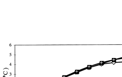
4. Numerical illustration
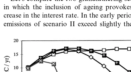
Below, a number of figures are presented for the scenarios. Fig. 2 depicts the interest rate, defined for the years between two periods starting at 2020. Fig. 3 and Fig. 4 present the flow vari-ables CO2 emission price and net CO2 emission,
each describing a flow during the periods 2000 – 2020, 2020 – 2040 and so forth. In these graphs, the periods are identified with the corresponding central years, 2010, 2030, etc. Fig. 5 and Fig. 6 illustrate the state variables CO2 concentration
and global mean temperature, defined for the years between two periods: 2000, 2020, etc.
Fig. 2 shows the interest rate evolution for each of the four scenarios. Three results require special attention. All three results confirm the inferences drawn in Section 3 from Fig. 1. First, comparing the interest rates between scenarios I+II and III+IV in 2020, we see that grandfathering the environmental resource implies initially an interest rate of close to 2 percent per year higher than in the trust fund case. Secondly, the intergenera-tional distribution of the property rights over the environmental resource has an even stronger im-pact on the long-term value of the interest rate. Sharing the property rights with future genera-tions, instead of grandfathering it, decreases the interest rate from 7.3 to 2.9 percent per year in 2200 (scenario I vs. III), when the population is not assumed to age. Including the demographic
Fig. 2. Interest rate for the period 2000 – 2200. change, we find that sharing the property rights decreases the interest rate from 2.5 to 0.5 percent per year in 2200 (scenario II vs. IV). Thirdly, comparing the scenarios with and without ageing, one concludes that ageing decreases the future interest rate substantially, from 7.3 to 2.5 percent in 2200 under grandfathering (scenario I vs. II), and from 2.9 to 0.5 percent in 2200 (scenario III vs. IV) if property rights are shared with future generations. The figure reveals the importance of both demographic changes and environmental policies for the long-term evolution of the interest rate. To compare our results with the results obtained with a typical dynastic model, we note that in a dynastic model the assumed slow-down of per capita economic growth from 2 percent per year in 2000 to zero in 2200 would cause a decrease in the interest rate of about 3 percent per year: Dr:gDg, where g=1/r=1.5 and Dg=2 percent per year. Except for the first scenario, all other scenarios show a much stronger decrease in the interest rate than the levelling of economic growth can account for. Overall, the figure unde-niably reveals that assumptions on demography and environmental policies substantially affect the interest rate, contrary to what is suggested in the literature (Stephan et al., 1997; Manne, 1999).
Fig. 3. CO2emission price for the period 2000 – 2200.
of scenario I because of the ageing of the popula-tion: the resulting increase in life-cycle savings and the associated increase in the man-made capi-tal stock produces more carbon dioxide than in an economy without ageing. In the 22nd century, however, the small effect of this demographic change is dominated by the increasing difference in the carbon dioxide price of these two scenarios. The steady rise in emission prices in scenario II outweighs the increase in emissions resulting from economic growth. This leads to a rapid decrease of emissions in scenario II, whereas in scenario I only a modest emission reduction takes place at the end of the 22nd century. In scenario II, cumu-lative emissions from today up to the year 2100 amount to about 1450 GtC, which is comparable with the corresponding IPCC IS92a scenario (IPCC, 1992). By the year 2200, net emissions will have attained the level of zero.
Altering the analysis from a ‘victims pay’ to a ‘polluters pay’ perspective, by the introduction of a trust fund, substantially shifts upwards the car-bon dioxide emission price curve. In the case of the ageing scenario, the increase is already visible in the first period, whereas it becomes apparent in the second half of the 21st century for the no ageing case. The inclusion of ageing has a consid-erable effect on the emission price evolution. If no ageing is considered, the trust fund emission price remains neatly between the two grandfathering scenarios over the entire time lapse studied. This applies as well to the emission levels, insofar as the 22nd century is considered. If ageing is in-cluded in the calculations (scenario IV), the emis-sion price increases rapidly to 400 US$/tC in less than a century. Scenario IV does not limit the expansion of net emissions in the medium term (up to 2030), leaving present generations the pos-sibility to adapt and to develop alternative energy sources. After 2050 net emissions decrease rapidly, and by 2080 a complete substitution of fossil fuel energy carriers by carbon-free energy sources has taken place.
As can be seen from a comparison between Fig. 4 and Fig. 5, CO2 concentration levels in the
atmosphere lag behind CO2 emission patterns. In
turn, an inspection of Fig. 6, depicting the global average temperature increase relative to the pre-in this scenario (see Fig. 4) are roughly stable on
the time scale considered. An autonomous in-crease in energy efficiency (AIEE) and an au-tonomous expansion of backstop technologies, assumed in the benchmark scenario (see the para-graph directly following Eq. (11)), mainly explain this approximately stable emission level. The rela-tively small reduction in emissions close to the year 2200 is induced by the expected emission price increase around that date for this scenario. It should be understood, however, that these esti-mates are dependent on the benchmark assump-tions made. Chakravorty et al. (1997), for example, assume an autonomous decline of fossil fuel energy use before 2100 because of competitive solar energy supply.
Let’s compare the two grandfathering scenarios in which the inclusion of ageing provokes a de-crease in the interest rate. In the early periods, net emissions of scenario II exceed slightly the levels
Fig. 5. Atmospheric CO2 concentration for the period 2000 – 2200.
5. Conclusion
The figures presented in this paper illustrate the importance of taking into account two phenom-ena, which may affect future interest rates, but are for methodological reasons often neglected in dy-nastic models. The first is the expected modifica-tion in life expectancy of the world populamodifica-tion. This change is exogenous to the policy maker. The second is the possibility of designing an in-strument for preserving the natural environment, such as grandfathering or the establishment of a trust fund. The choice for policy instruments is open for the policy maker, and in this way, he may influence the interest rate.
Our purpose has been not so much to present yet another set of numbers, adding to the many results which have been published already on the subject of global warming and greenhouse gas mitigation. Our main message is to emphasise that, in general, a cautious use and interpretation of results on this matter is required. It is shown that the results are highly sensitive for the interest rate, which in turn depends on parameters that represent demography and environmental policy. For economic modelling, it is recommended not to employ a rigid discounting relation that links the interest rate to other fixed parameters.
This judgement puts into question the use of dynastic IAMs. In the standard dynastic model with time-additive discounted welfare functions, and with a constant RPTP, the future interest rate depends on a limited number of parameters. These parameters are usually calibrated on his-toric data, and the results of dynastic models are often interpreted to suggest that a choice for environmental conservation is at odds with effi-ciency. The dynastic model, however, over-sim-plifies the analysis and misleads the responsibility of present policy makers. By the assumption of a flexible discounting relation, an OLG analysis can provide insights which can be attained with difficulty from dynastic models. The trust fund described in this paper is a possible step towards the formulation of an instrument that may estab-lish a combination of both efficiency and conservation.
industrial level over the interval 2000 – 2200, shows that the mean temperature lags behind the CO2 concentration level. Fig. 5 and Fig. 6 show
that, regarding the carbon dioxide concentration and average global temperature increase, the first three scenarios nearly coincide during the forth-coming 150 years. Only scenario IV, in which not only future generations are given a share of the environmental resource value, but in which also the expected demographic change occurring in the 21st century is accounted for, succeeds in starting reducing temperatures slightly in the 22nd cen-tury. The environmental policy of scenario IV endogenously adjusts the interest rate to a level that supports a resource conservation.
Acknowledgements
Part of this research has been carried out under EU-project ENV4-CT98-0810, ‘An Integrated As-sessment of European Interests and Strategies in the Climate Negotiations Process Beyond Kyoto’ of the European Union DG-XII. Reyer Gerlagh is grateful to Michiel Keyzer for the supervision when developing the ALICE model (several ver-sions) as part of his Ph.D. research. Both authors thank three anonymous referees for their con-structive and comprehensive suggestions on the presentation and contents of this paper. The au-thors are, of course, entirely responsible for all remaining errors.
References
Auerbach, A.J., Kotlikoff, L.J., Hagemann, R.P. et al., 1989. The economic dynamics of an ageing population: the case of four OECD countries, OECD Economic Studies 12, OECD, Paris.
Azar, C., Sterner, T., 1996. Discounting and distributional considerations in the context of global warming. Ecological Economics 19, 169 – 184.
Barro, R.J., 1974. Are government bonds net wealth? Journal of Political Economy 82, 1095 – 1117.
Blanchard, O.J., Fischer, S., 1989. Lectures on macroeconom-ics. MIT Press, MA, Cambridge.
Broome, J., 1992. Counting the costs of global warming. White Horse Press, MA, Cambridge.
Chakravorty, U., Roumasset, J., Tse, K., 1997. Endogenous substitution among energy resources and global warming. Journal of Political Economy 105, 1201 – 1234.
Clark, C.W., 1997. Renewable resources and economic growth. Ecological Economics 22, 275 – 276.
Cline, C.W., 1992. The Economics of Global Warming. Insti-tute for International Economics, Washington, DC. Davies, J.B., 1981. Uncertain lifetime, consumption, and
dis-saving in retirement. Journal of Political Economy 89 (3), 561 – 577.
Epstein, L.G., 1987. The global stability of efficient intertem-poral allocations. Econometrica 55, 329 – 355.
Farmer, M.C., Randall, A., 1997. Policies for sustainability: lessons from an overlapping generations model. Land Eco-nomics 73 (4), 608 – 622.
Gale, D., 1973. Pure exchange equilibrium of dynamic eco-nomic models. Journal of Ecoeco-nomic Theory 6, 12 – 36. Geanakoplos, J.D., Polemarchakis, H.M., 1991. Overlapping
generations, Hildenbrand, W. and Sonnenschein, H. (Eds.), Handbook of Mathematical Economics IV, Ch. 14, North-Holland, Amsterdam.
Gerlagh, R., 1998a. The efficient and sustainable use of envi-ronmental resource systems. Thela Thesis, Amsterdam. Gerlagh, R., 1998b. ALICE 1; an Applied Long-term
Inte-grated Competitive Equilibrium model. W98-21, IVM, In-stitute for Environmental Studies, Amsterdam.
Gerlagh, R., Keyzer, M.A. Sustainability and the intergenera-tional distribution of natural resource entitlements. Journal of Public Economics, forthcoming.
Gerlagh, R., van der Zwaan, B.C.C., 1999. Sustainability and discounting in Integrated Assessment Models, Nota di Lavoro, 63.99, Fondazione Eni Enrico Mattei (FEEM), Milan, Italy.
Gerlagh, R., van der Zwaan, B.C.C., Overlapping generations versus infinitely-lived-agent, the case of global warming. In: Howarth, R. and Hall, D. (Eds.), in: Advances in Environmental Resources, JAI Press, Stamford, CT, USA, forthcoming..
Howarth, R.B., 1998. An overlapping generations model for climate-economy interactions. Scandinavian Journal of Economics 100, 575 – 591.
Howarth, R.B., Norgaard, R.B., 1992. Environmental valua-tion under sustainable development. American Economic Review 82, 473 – 477.
Hurd, M.D., 1989. Mortality risk and bequests. Econometrica 57 (4), 779 – 813.
IPCC (Intergovernmental Panel on Climate Change), 1992. Climate change 1992; The supplementary report to the IPCC scientific assessment. Cambridge University Press, Cambridge.
IPCC, 1996a. Climate change 1995; Impacts, adaptations and mitigation of climate change: scientific-technical analyses. Cambridge University Press, Cambridge.
IPCC, 1996b. Climate change 1995; Economic and social dimensions of climate change. Cambridge University Press, Cambridge.
Kehoe, T.J., 1991. Computation and multiplicity of equilibria. In: Hildenbrand, W., Sonnenschein, H. (Eds.), Handbook of Mathematical Economics, part IV, Ch. 38, North-Hol-land, Amsterdam.
Koopmans, T.C., 1960. Stationary ordinal utility and impa-tience. Econometrica 28, 287 – 309.
Koopmans, T.C., Diamond, P.A., Williamson, R.E., 1964. Stationary utility and time perspective. Econometrica 32, 82 – 100.
Krautkraemer, J.A., 1985. Optimal growth, resource amenities and the preservation of natural environments, Review of Economic Studies, LII: 153 – 170.
Lucas, R.E., Jr., Stokey, N.L., 1984. Optimal growth with many consumers. Journal of Economic Theory 32, 139 – 171.
Maier-Reimer, E., Hasselmann, K., 1987. Transport and stor-age of CO2in the ocean — an inorganic ocean-circulation carbon cycle model. Climate Dynamics 2, 63 – 90. Manne, A.S., 1999. Equity, efficiency, and discounting. In:
Manne, A.S., Mendelsohn, R., Richels, R., 1995. MERGE, A model for evaluating regional and global effects of GHG reduction policies. Energy Policy 23, 17 – 34.
Manne, A.S., Richels, R., 1995. The greenhouse debate; eco-nomic efficiency, burden sharing and hedging strategies. Energy Journal 16, 1 – 37.
Nordhaus, W.D., 1994. Managing the global commons. MIT Press, MA, Cambridge.
Nordhaus, W.D., Yang, Z., 1996. A regional dynamic general equilibrium model of alternative climate-change strategies. American Economic Review 86, 741 – 765.
Peck, S.C., Teisberg, T.J., 1992. CETA: a model for carbon emissions trajectory assessment. Energy Journal 13, 55 – 77. Roberts, K.W.S., 1980. Interpersonal comparability and social
choice theory. Review of Economic Studies XLVII, 421 – 439.
Stephan, G., Mu¨ller-Fu¨rstenberger, G., Previdoli, P., 1997. Overlapping generations or infinitely-lived agents: intergen-erational altruism and the economics of global warming. Environmental and Resource Economics 10, 27 – 40. Tol, R.S., 1995. The Damage Costs of Climate Change
To-ward More Comprehensive Calculations. Environmental and Resource Economics 5, 353 – 374*.
World Bank, Bos, E., Vu, M.T., Massiah, E., Bulatao, R.A. (Eds.), 1994. World population projections 1994 – 95 edi-tion; estimates and projections with related demographic statistics. Johns Hopkins University Press, Baltimore, MD, USA.