VISUALIZATION OF MOBILE MAPPING DATA VIA PARALLAX SCROLLING
D. Eggerta, E. C. Schulzeb
Institute of Cartography and Geoinformatics, Leibniz Universit¨at Hannover, Germany -a
[email protected],[email protected]
Commission III, WG III/5
KEY WORDS:Point-cloud, Visualization, Mobile Mapping, Parallax Scrolling, Image-based rendering, Real-time rendering
ABSTRACT:
Visualizing big point-clouds, such as those derived from mobile mapping data, is not an easy task. Therefore many approaches have been proposed, based on either reducing the overall amount of data or the amount of data that is currently displayed to the user. Furthermore, an entirely free navigation within such a point-cloud is also not always intuitive using the usual input devices. This work proposes a visualization scheme for massive mobile mapping data inspired by a multiplane camera model also known as parallax scrolling. This technique, albeit entirely two-dimensional, creates a depth illusion by moving a number of overlapping partially transparent image layers at various speeds. The generation of such layered models from mobile mapping data greatly reduces the amount of data up to about 98% depending on the used image resolution. Finally, it is well suited for the panoramic-fashioned visualization of the environment of a moving car.
1. INTRODUCTION
The visualization of large amounts of data usually yields various problems. Either the user is overwhelmed by the sheer volume of information and therefore maybe missing the features important to him or the hardware displaying the data reaches its limit and is unable to provide interactive framerates. One way to face these problems is to reduce the amount of data (or generalize it) to such an extent that the above constraints are met.
One way of generalization is dimensionality-reduction. In case of mobile mapping we have to deal with colored three dimensional point-clouds. Reducing the data about the height property for example, results in map-like representation as shown in figure 1.
Figure 1: 2D map derived from mobile mapping point-cloud by eliminating the height property.
While this kind of visualization gives a nice overview of the scene it also eliminates all uprising structures like facades. In order keep the facade structures the height property has to be kept as
well. An alternative property to reduce would be the depth prop-erty. Since this property depends on the point of view (POV), eliminating the depth results in a limitation of possible POVs. This fact raises two questions, first which POVs shall be used and second how does it impact the navigation through the data.
Since the visualization aims for displaying mobile mapping, it felt natural using the acquisition vehicle’s track as possible POVs. Restricting the virtual camera to those POVs enables the visual-ization to handle areas of missing information in a sophisticated manner as discussed in chapter 5. The impact on the navigation is noticeable. The scene can only be seen from the given trajectory points, so the only real navigation option the user has is to move forward or backward on the trajectory. Furthermore the viewing direction is also fixed, which means only one street-side can be watched at a time. While this appears to be a significant limita-tion it simplifies the navigalimita-tion through the rather complex data as well. This simple navigation enables even non experienced users to easily browse through the mobile mapping data. Which makes the proposed visualization scheme more comparable to systems like Google’s Streetview (Vincent, 2007) and Microsoft’s Street-slide (Kopf et al., 2010) as to systems visualizing a complete 3D city model.
Finally, in order to regain at least a sense or an illusion of depth the concept of parallax scrolling comes into play. Instead of en-tirely eliminating the depth property it is only clustered into dis-crete values, resulting in various depth layers. Rendering those layers on top of each other, as shown in figure 2 gives an illusion of depth which improves the quality of visualization compared to an entirely flat one, as shown in figure 1.
2. RELATED WORK
Over the years the processing and visualization of large point-clouds have been addressed by various publications.
In general most approaches can be classified into two categories. First the point-clouds can be generalized into simpler models with a lower level of detail (LOD). This reduces the amount of data significantly, but might remove relevant features from the data. One example from this category was published by (Wahl et al., 2005), where planes within a point-cloud are identified and points belonging to those planes are projected onto texture rep-resentations. This is based on the idea of exchanging geometry information with texture information which increases the render-ing speed. This is also often referred to as image-based repre-sentations for reducing the geometric complexity. (Jeschke et al., 2005) gives good overview of such approaches. In contrast to purely point based data in case of mobile mapping, impostors based methods like in (Wimmer et al., 2001) usually use 3D mesh models as their input data. The creation of such meshes are out of the scope of this work and thus using impostors is not a viable option, while the general idea will be applied in the presented work.
The second category simply reduces the data, in case of point-clouds the number of points, that is displayed at a time, e.g. by skipping points or regions that are currently not visible on screen. In case the points become visible they are loaded into memory, while the points and regions becoming invisible are dropped from the memory. Those approaches are usually referred to as out-of-core methods. In the end methods fusing both approaches (gener-alized models and out-of-core techniques) do also exist, render-ing far away objects with a low LOD, while increasrender-ing the LOD in case the objects are getting closer. (Richter and D¨ollner, 2010) and (Gobetti and Marton, 2004) discuss two varieties of such ap-proaches.
Since this work uses the concept of parallax scrolling which is based on image-based rendering, it belongs to the first domain of generalization of point-clouds.
Occlusions are a major problem when it comes to deriving mod-els from point-cloud data. As the texture images are derived from the recorded scan-points, they only convey information that was observed by the corresponding laser. Objects not reflecting the laser beam (e.g. windows) as well as objects or areas, occluded by other foreground objects do not appear in the generated im-ages. Since the images have to be transparent for the parallax scrolling rendering, the missing areas result in transparent holes. Those holes can be closed by interpolation, either in the original point-cloud like shown in (Wang and Oliveira, 2007) or in the re-sulting image as shown in (Efros and Leung, 1999). But as the actual origin is not entirely known, interpolation could lead to an overall wrong model. The restricted virtual camera dictated by the used visualization scheme allows to deal with those holes in different manners. Instead of filling them up they can also be hid-den in more or less the same way they were hidhid-den from the laser beam.
3. PARALLAX SCROLLING
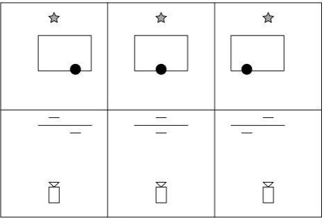
Parallax Scrolling is a visualization method, which creates a depth illusion in an animated, two dimensional scene. For this it uses multiple layers of two dimensional graphics, which are displayed on top of each other, thus forming a single image for the camera, which looks down at the top of the stack. In order to simulate a camera movement, each layer is moved at its own speed, instead
of moving the camera it self. Figure 3 elucidates this by showing a series of three pictures with layers moving at different speeds.
Figure 3: Sketch of parallax scrolling scene with simulated cam-era movement from left to right. Upper row: The images that the camera sees. Lower row: The camera looking at the layers.
3.1 Mathematics Behind Parallax Scrolling
For a general visualization with parallax scrolling one needs a sequence L of layersli. Let L = hl1, l2, . . . , lni be ordered
such thatl1is at the top of the stack, meaning closest to the cam-era, andln is at the bottom of the stack, meaning the farthest
away from the camera. Each layerihas, next to its image data, a
two-dimensional positionp~i =
In order to display the entire scene, we must render each layer of the stack beginning at the bottom and ending at the top. This way the rendered image will only contain pixels, which are not occluded by other layers.
As mentioned before the camera is always steady, hence to
vir-tually move the Camera by∆ =~
layer’s position in respect to its speed instead. The new positions
~
pi′are calculated as follows:
~
pi′=p~i−vi·∆~ (1)
3.2 Perspective Parallax Scrolling
Simply rendering various image layers on top of each other re-sults in an orthogonal projection, which might appear quite un-natural. In order to create a more appealing perspective correct parallax scrolling, we need to calculate the layer-speedsvi.
Fur-thermore, we also need to calculate a scaling factorsifor each
layer, to simulate the fact that an object looks smaller the bigger the distance to the observer is.
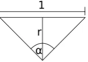
Letαbe the horizontal aperture of the camera. Also letdibe
the distance of the i-th layer to the camera. Now we calculate the distancerat which one length unit in the model matches one length unit in the image (see figure 4).
r= 1
1
r
α
Figure 4: Sketch of the calculation ofr.
half as big in both dimensions. Therefore the scaling factorsiis
calculated as follows:
si=
r di
(3)
The same argument can be used to calculate the speedvi, which
means thatvi=si.
In order to finally draw the scene the new corner positions for each layer have to be calculated. Let~pbe a corner position of the i-th layer. Also, let~cbe the camera position andz be the camera zoom factor. The new position of the corner is calculated as follows:
~
p′=z·(si·~p−vi·~c) =z·si·(~p−~c) (4)
With the known corners the layer image can be scaled and drawn accordingly.
4. MODEL GENERATION
Visualizing the mobile mapping data using the parallax scrolling technique requires the data to be ordered in layers. Each layer represents a distinct depth or depth-range. Considering mobile mapping relevant layers can be (in ascending distance from the acquisition vehicle) cars (on the road), parking cars, street furni-ture (traffic signs, traffic lights, trees, etc.), pedestrians and finally the building facades.
4.1 Identification of relevant layers
In order to identify those relevant layers mentioned above many approaches are feasible. This paper discusses two approaches (geometry-based and semantic-based).
The first method is purely based on the geometry of the point-cloud input data. First of all the acquisition vehicle’s track is simplified, while the resulting track segments are used to find relevant layers. To this end a buffer around each segment is de-fined and two histograms (one for each street-side) reflecting the distances of all scan-points within this buffer towards the corre-sponding track segment are created. Figure 5 shows a typical distance histogram.
While the maximum peak usually represents the building facade layer, all minor peaks represent object layers. In order to extract the position and size of each layer the current maximum peak is used as the start value, while all neighboring distances, to the left as well as to the right, will be assigned to this maximum peak until a value below a given threshold is found and a minimum number of points had been assigned. After removing all assigned values from the histogram the process recursively identifies the remaining layers by again starting at the maximum peak value. Since the building facade layer is likely to be the most distant rel-evant layer all values behind the first maximum peak are assigned
Figure 5: Distance histogram of all points on a single street-side for a given track segment.
Figure 6: Distance histogram with color-encoded relevant layers.
to this layer. Figure 6 shows a possible result, with all identified relevant layers.
The second, semantic-based approach is based on segmenting and classifying the point-cloud. Our segmentation method first extracts all ground points from the point-cloud using a normal-based region-growing. This leaves all remaining objects uncon-nected, hence all objects are again segmented by region-growing. Depending on the desired visualization scenario the all segmented objects have to be classified. Within the scope of this work we merely classified the objects intobuilding/facadeandother. Fi-nally the relevant building layer is derived from the classified building objects by detecting the major facade plane using the RANSAC, see (Fischler and Bolles, 1981), plane-fit method. All remaining objects are represented by a track-segment parallel layer passing through the object’s center of mass.
4.2 Final Layer-Model
After the relevant layers have been detected the corresponding texture representation is generated by projecting the associated points onto the respective layer planes. Depending on the point-cloud’s density and the used image-resolution the resulting im-age can appear quite sparse. In order to face this intermediate pixels can be interpolated accordingly. Both the point to plane projection as well as the pixel interpolation are in detail covered by (Eggert and Sester, 2013). An exemplary image is shown in figure 7.
Figure 7: Resulting texture image representing a single layer
5. HIDING BLIND SPOTS AND HOLE-FILLING
During the mobile mapping process it will often be the case, that some objects are partially occluded by others, e.g. a parking car in front of a house. Since the LiDAR’s laser beams do gener-ally not pass through solid objects, this leads to volumes of no information.
The camera movement in our model is constrained to the trajec-tory of the mobile mapping system. Therefore it is easy to as-sume, that these blind spots would not show up in the visualiza-tion. But in contrast to the real world objects the visualized ones are flattened. As figure 8 points out, this assumption doesn’t hold in the parallax scrolling visualization.
Figure 8: Left: The car is blocking the camera from seeing the blind spot on the wall. Right: The lack of depth on the car enables the camera to see the blind spot.
In order to rectify this problem by making the blind spots in-visible again, the positions of the occluding objects have to be altered. The first step is finding the corresponding occluders for the holes. This is done by first finding the holes in the textures of the objects, which are not in the topmost layer. For this we determine the connected components of the texture in regards to pixels, which are marked as holes, using a two-pass algorithm as described by (Azriel Rosenfeld, 1966). Then we calculate the bounding boxes of these connected components and transform them from texture space to model space. The corresponding oc-cluder for a hole is now the closest object that lies completely in front of the bounding box. Now that we know the holes for each occluding object, we can adjust the position, such that the holes will not be visible in the visualization. For this we show two variants in this paper:
1. Static hiding
2. Movable hiding
5.1 Static Hiding
The basic idea is, that the hole is not visible, if its occluding ob-ject moves at the same speed (they do not move relative to each other, hence naming it ”static”). In order to achieve this, the ob-ject needs to be pushed back, so that it is just in front of the hole,
as shown in figure 9. It must not be put in the same layer as the hole to avoid confusion in the drawing order. If the object cor-responds to more than one hole, the one nearest to the camera is chosen, otherwise the object would be placed behind a hole, which makes hiding it impossible.
Figure 9: Left: The original scene. Right: The scene with the use of static hiding.
While this variant does fulfill its task of hiding the blind spots, it performs radical changes to the scene. Often foreground ob-jects are pushed noticeably far back, being practically wallpa-pered onto another object.
5.2 Movable Hiding
Static hiding often pushes objects too far back. In the original scene those objects are not pushed back far enough. From these observations we can conclude, that there must be an optimal dis-tance, at which the occluder is just near enough to the hole to hide it, but can still move relative to it. Finding and relocating the occluding object to this distance is the task of movable hiding.
In order to determine that distance we first assume, that the hole lies centered behind the occluding object, which is depicted in figure 10. In that figure the camera is placed in two positions, such that the hole is just outside of the camera image. The goal is to calculate the distanced, which determines how far in front of the hole the occluder must be placed.
b
α α
β r
d
q
Figure 10: Birds-eye view on the movable hiding situation.
Let αbe the aperture of the camera, b the width of the hole andq the width of the occluder. The edges of the two camera cones meet behind the hole and form a triangle with the hole, one with the desired position of the occluder and one with the cam-era movement line. It is obvious, that the angleβat that point is equal toα. Withαandbwe can calculate the distancerbetween the triangle point and the hole.
r= b 2·cot
α
2
(5)
We can also calculate the distancer+dto the desired position of the occluder.
r+d= q 2·cot
α
2
Now we can determinedthrough simple subtraction.
d=q 2·cot
α
2
−b 2·cot
α
2
= q−b 2 ·cot
α
2
(7)
The distance to the camera of the occluder can now simply be set to the distance to the camera of the hole minusd.
If the hole is not centered behind the occluder, we can artificially enlarge the hole to one side until the state is fabricated. Also, if the occluder corresponds to more than one hole, we calculate the new distances to the camera for every hole and take the biggest distance. If that distance is further away than the nearest hole, we use static hiding instead.
5.3 Hole-Filling
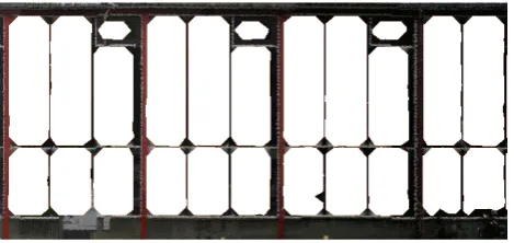
Another fact decreasing the visualization quality are holes that are not caused by occlusion. Empty areas that are not occluded are usually caused by materials that do not reflect the laser beams. Glass is such an material, so windows often result in rectangular holes in the facades texture images as depicted by figure 11.
Figure 11: Building facade containing holes caused by windows.
Detecting and classifying those holes/windows within the image data is a bit out of scope of this paper and is already addressed by various other publications like (Ali et al., 2007). As mentioned earlier, our approach uses a connected component analysis in or-der to find the corresponding holes. The actual filling will be discussed in the following in more detail. The algorithm distin-guishes between two types of holes, small and big ones.
Small holes are probably not caused by windows rather by an-other material not reflecting the laser beam. That’s why small holes are filled by interpolation. As the first step the colored bor-der pixels of the hole are determined. Based on the location and color of those pixels two dimensional function is approximated for each color channel. In the end a color for all pixels is derived based in the determined functions, while the pixel coordinates are used as input values.
Big rectangular holes, in contrast to small holes, are very likely caused by windows. Since the border of those holes are repre-sented by the corresponding window frames, interpolating the color between those is not a good idea, because the frame’s color usually has nothing to do with the color of the window’s glass. Therefore those holes are covered by a gray rectangle mimicking the window’s glass. For a more natural visualization some noise is added as well. The result is shown in figure 12. While the three small holes in the upper part are filled using the approximated color functions, the big holes are covered by gray rectangles.
Figure 12: Building facade with filled holes.
6. IMPLEMENTATION AND RESULTS
The implementation of the visualization was done in Java, using the ”Lightweight Java Game Library” (Lightweight Java Game Library, 2013) for its OpenGL bindings. While the usage of a 3D-capable graphics library is in no way necessary, as indeed no 3D-functions of OpenGL were used, we used it for its efficient handling and rendering of textured faces.
The first step when loading the scene is to prepare it for efficient rendering. This consists of translating the scene such that the camera starts of in the middle of it, scaling the layers by their distances and calculating their speeds. The translation is done by calculating the scenes 2D-bounding box (ignoring the depth), determining the position of its middle and translating every layer, which means every quad in a layer, such that the new middle
posi-tion of the bounding box is at
0 0
. Scaling and speed calculation
are done as described in chapter 3.
After that, the quads of every layer, as well as their textures, are uploaded into OpenGL memory. Each quad consists of four ver-tices, which consist of their two dimensional spacial positions, as well as their two dimensional texture coordinates. Because OpenGL has a limitation on the maximum size of a texture, we can not just combine every quad of a layer into one big quad.
The rendering of the scene is done as described in chapter 3. At first we clear the screen. Then the stack of layers is rendered bot-tom to top. Each layer is rendered by rendering all its contained quads, which are stored as vertex buffer objects and references to their textures. The translation of each layer with regards to the simulated camera position is done in the vertex shader and works as in equation (4), with a few exceptions. The vertex positions are already scaled according to their layers distance. Also, OpenGLs screen coordinates are always∈[−1,1]for both dimensions, no matter if the screen is actually square or not. Therefore it is nec-essary, to add the aspect ratio as a factor for the y-coordinate. The fragment shader just does a texture lookup.
6.1 Results
Moreover, the figure also reveals various problems not necessar-ily related to the proposed visualization scheme. For instance, some building parts mainly in the upper region are missing. This is caused by the fact that the acquisition vehicle was passing to closely by the corresponding building, which means the cameras taking the pictures used for coloring the point-cloud were also very close. The closer the camera is the less of the buildings fa-cade is covered by the resulting image, which results in missing colors for the corresponding points. Furthermore, the shown tree in the center shows also weird colors. This results from the fact that the used camera might not have been calibrated correctly and the tree points are mapped to pixels in between the tree branches. This are basically pixels from the sky and therefore often blue or white.
Figure 13: Resulting parallax scrolling visualization.
One motivation for the proposed visualization scheme was the inability of modern hardware to render massive mobile mapping point-clouds in real-time. The rendering of a single frame took less than a millisecond for the implemented prototype on a mod-ern computer, which allows a theoretic framerate of 1000 fps, enabling even low-end devices or web-based applications.
7. CONCLUSIONS AND FUTURE WORK
This work introduced a new visualization scheme for massive mobile mapping data based on the parallax scrolling technique. An overview of layered models are derived from the mobile map-ping point-cloud data, especially the identification of relevant lay-ers is discussed. As shown in chapter 5. the presented approach enables interesting ways of dealing with holes caused by occlu-sion, by recreating the original occlusion situation in the visu-alized scene. This hiding instead of interpolating bypasses many problems caused by interpolation. Finally an OpenGL-based pro-totype implementing the proposed scheme was realized. Even with a minimum number of two layers the illusion of depth was clearly perceptible, while amplified by the use of more layers. As the results indicate a real-time rendering of even big datasets is rather unproblematic, and therefore applicable for many scenar-ios, including even web-based visualizations.
Alongside the actual visualization many issues have to be ad-dressed in later research. In order to enhanced the visualiza-tion quality the coloring of the original point-cloud has to be im-proved, e.g. applying a fine-tuned mobile mapping camera cali-bration as presented in (Hofmann et al., 2014). Moreover more sophisticated layered model building techniques will be evalu-ated. Another approach to enhance the depth illusion beside the parallax effect is the use of bump or displacement mapping, which could be integrated into future prototypes. While the discussed static and movable hiding schemes present rather basic concepts, more sophisticated approaches are possible, which will also be elaborated in future research.
REFERENCES
Ali, H., Seifert, C., Jindal, N., Paletta, L. and Paar, G., 2007. Window detection in facades. In: Image Analysis and Process-ing, 2007. ICIAP 2007. 14th International Conference on, IEEE, pp. 837–842.
Azriel Rosenfeld, J. L. P., 1966. Sequential operations in digital picture processing.
Efros, A. and Leung, T., 1999. Texture synthesis by non-parametric sampling. In: Computer Vision, 1999. The Proceed-ings of the Seventh IEEE International Conference on, Vol. 2, pp. 1033–1038 vol.2.
Eggert, D. and Sester, M., 2013. Multi-layer visualization of mo-bile mapping data. ISPRS Annals of Photogrammetry, Remote Sensing and Spatial Information Sciences.
Fischler, M. A. and Bolles, R. C., 1981. Random sample con-sensus: A paradigm for model fitting with applications to im-age analysis and automated cartography. Commun. ACM 24(6), pp. 381–395.
Gobetti, E. and Marton, F., 2004. Layered point clouds: a simple and efficient multiresolution structure for distributing and render-ing gigantic point-sampled models. Computers & Graphics 28(6), pp. 815–826.
Hofmann, S., Eggert, D. and Brenner, C., 2014. Skyline matching based camera orientation from images and mobile mapping point clouds. ISPRS Annals of Photogrammetry, Remote Sensing and Spatial Information Sciences II-5, pp. 181–188.
Jeschke, S., Wimmer, M. and Purgathofer, W., 2005. Image-based representations for accelerated rendering of complex scenes. In: Y. Chrysanthou and M. Magnor (eds), EURO-GRAPHICS 2005 State of the Art Reports, EUROEURO-GRAPHICS, The Eurographics Association and The Image Synthesis Group, pp. 1–20.
Kopf, J., Chen, B., Szeliski, R. and Cohen, M., 2010. Street slide: Browsing street level imagery. ACM Transactions on Graphics (Proceedings of SIGGRAPH 2010) 29(4), pp. 96:1 – 96:8.
Lightweight Java Game Library, 2013.
http://www.lwjgl.org/index.php.
Richter, R. and D¨ollner, J., 2010. Out-of-core real-time visualiza-tion of massive 3d point clouds. In: 7th Internavisualiza-tional Conference on Virtual Reality, Computer Graphics, Visualisation and Inter-action in Africa, pp. 121 – 128.
Vincent, L., 2007. Taking online maps down to street level. Com-puter 40(12), pp. 118–120.
Wahl, R., Guthe, M. and Klein, R., 2005. Identifying planes in point-clouds for efficient hybrid rendering. In: The 13th Pacific Conference on Computer Graphics and Applications, pp. 1–8.
Wang, J. and Oliveira, M. M., 2007. Filling holes on locally smooth surfaces reconstructed from point clouds. Image Vision Comput. 25(1), pp. 103–113.