MULTI-DIMENSIONAL QUALITY ASSESSMENT OF PHOTOGRAMMETRIC
AND LIDAR DATASETS BASED ON A VECTOR APPROACH
M. Mohameda
, T. Landesa
, P. Grussenmeyera
, W. Zhangb
a
INSA Strasbourg, ICube Laboratory UMR 7357, Photogrammetry and Geomatics Group Strasbourg, France- (mostafa.mohamed, tania.landes, [email protected]) b
State Key Laboratory of Remote Sensing Science, Beijing Key Laboratory of Environmental Remote Sensing and Digital City, School of Geography, Beijing Normal University, 100875 Beijing, China - ([email protected])
KEY WORDS:Optical imagery, LiDAR, 3D building modeling, Quality assessment, RMSE, Surface indices, Volume indices.
ABSTRACT:
The production of 3D city models requires the reconstruction of individual 3D building models. As the performance of data acquisition methods improves, the quality evaluation of building models in 3D has become an important issue. The main objective of the presented work is to introduce a multi-dimensional approach for assessing the quality of 3D building vector models. This approach performs assessments in 1D, 2D and 3D by comparing calculated building models to their reference. For 1D assessment, homologous points in two buildings to be compared are analyzed. For 2D assessment, homologous planes enter in the evaluation process. Quality of the planes under study is assessed by calculating a set of indices in vector format. For 3D assessment, building models are considered as one object. Quality of the buildings is assessed by calculation of vector volumetric quality factors. These factors require the not trivial calculation of vector intersection volumes which calculation is presented in the paper. Intersection volume is defined by superimposing the building model to be tested with the reference one. The multi-dimensional vector assessment approach has been applied to evaluate the building models produced with three different reconstruction processes created from different types of datasets. The datasets are obtained by photogrammetry (UltraCam-X and Zeiss LMK cameras), by LiDAR, and also by integration of photogrammetric and LiDAR datasets. The 1D, 2D or 3D assessment approach allows highlighting the source of deviations in the tested buildings. The error budget affecting the final product is not only composed of errors due to the reconstruction algorithm. Also errors due to the quality of the raw data, the processing of LiDAR data, of aerial data and the shape of the produced buildings should be considered.
1 INTRODUCTION
Photogrammetric and LiDAR data are used since many years for the 3D reconstruction of objects such as buildings. These ap-plications need accurate data and methods in order to produce good results. Quality assessment is critical for 3D data produc-tion and is important for several reasons. Firstly, it may give im-portant information about deficiencies of an approach and may take place to help in focusing a further research activity. Sec-ondly, accuracy evaluation is needed in order to compare the re-sults of the different approaches and to convince a user (Schuster and Weidner, 2003). Several methods were presented in order to evaluate photogrammetric and LiDAR datasets. Calculation of Root Mean Square Errors (RMSE) for analyzing the precision of the complete 3D building is an interesting process. It shows the shifts between reference and test models in X, Y and Z direc-tions. (Grussenmeyer et al., 1994) proposed statistical techniques in order to calculate RMSE by point and line based assessment. Several approaches using quality factors for quality evaluation of building models were introduced ((McKeown et al., 2000), (Ra-gia, 2000)). Based on these, a further approach was developed, which introduced alternative quality measurements (Schuster and Weidner, 2003).
All accuracy assessments processes include three fundamental steps (Congalton and Kass, 2009). Firstly, the accuracy assess-ment sample should be designed. The sampling design issues are similar to those traditionally addressed by survey sampling methodology: how to choose sample in a cost-effective and at the same time statistically rigorous manner? Application of ba-sic sampling designs such as simple random, stratified random, systematic and cluster have been summarized in (Congalton and Kass, 2009). Secondly, data must be collected for each sam-ple; and finally, results must be analyzed. Because high qual-ity reference data are difficult and expensive to obtain, reference
model may be considered as error-free, more accurate than the test model, or with the same accuracy as the test model (Meidow and Schuster, 2005). Once the reference data are available, the assessment process can start.
Related works were done by the Photogrammetry and Geomatics Group at INSA-Strasbourg. In the context of assessing the quality of planes detection in a 3D building reconstruction process based on LIDAR data, several solutions have been suggested (Tarsha-Kurdi et al., 2008). For evaluating the quality of geometric facade models reconstructed from TLS data, (Landes et al., 2012a) sug-gested the use of quality factors and RMSE calculations. Also, the evaluation of characteristic planes extracted from digital air-borne sensors have been published in (Mohamed and Grussen-meyer, 2011). A new approach has been proposed for assessing 3D building models based on vector volumetric quality factors (Landes et al., 2012b). The main objective of the presented work is to introduce a multi-dimensional approach for evaluating the quality of 3D building models reconstruction. The approach used in this research is vector based.
2 ASSESSMENT OF 3D BUILDING MODELS
2.1 1D assessment
2.2 2D assessment
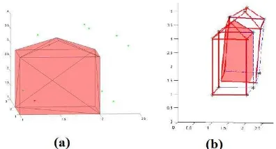
Our method to evaluate 2D data is based on the comparison of 3D planes of two building models (reference and test) by calcu-lating a set of indices. This approach uses well known quantities, as mentioned in (McKeown et al., 2000), (McGlone and Shufelt, 1994), (Ragia, 2000), (Schuster and Weidner, 2003) and (Lan-des et al., 2012b). These indices are namely the detection rate (ρd), the branch factor(ρb), the quality rate(ρq), miss factor (ρm), and false alarm rate(ρf)as summarized in Table 1. The principle idea of these indices is based on the relation between the reference surface area (Ar) and the tested surface area (At) as shown in Figure 1(a).
Figure 1: Relationship between reference and tested models in 2D (a) and 3D (b).
Quality factor Explanation
Detection rate: it is the ratio between the
ρd= Ar∩At
Ar intersection area between two planes and the
ρd∈[0 : 1] reference plane.ρd= 1means that the calculated polygon is perfectly superposed
Quality rate: it is the ratio between the
ρq=Ar∩At
Ar∪At intersection area between two planes and the
ρq∈[0 : 1] union of two planes.ρq= 1means that both polygons are perfectly superposed. Branch factor: it is the ratio of the part of the
ρb=ArAt\∩ArAt reference polygon which is not included
pb≥0 in the polygon under study and the intersection of the two polygons. Miss factor: Ratio of the part of the polygon
ρm=ArAr∩\AtAt being evaluated which is not included in a
ρm≥0 reference polygon and the intersection of the two polygons.
False alarm rate: it is the ratio of the part of
ρf=At\ArAr reference polygon which is not included
ρf≥0 in the polygon under study compared to the area of the reference polygon.
Table 1: Quality indices based on surface areas ratios.
2.3 3D assessment
Considering a building as one object to be evaluated, volume comparisons are rather appropriate than surface areas compar-isons. Therefore, the quality of buildings is assessed by the cal-culation of volumetric quality factors. The quality factors in 3D are deduced from the 2D quality factors and depend on ratios of volumes. These factors take into account the volume of the in-tersection as well as the union volume of two vector buildings. A first experiment has been introduced in (Landes et al., 2012b). The principle idea of these indices is based on the relation be-tween the reference volume(V r)and the tested volume(V t)as shown in Figure 1(b).
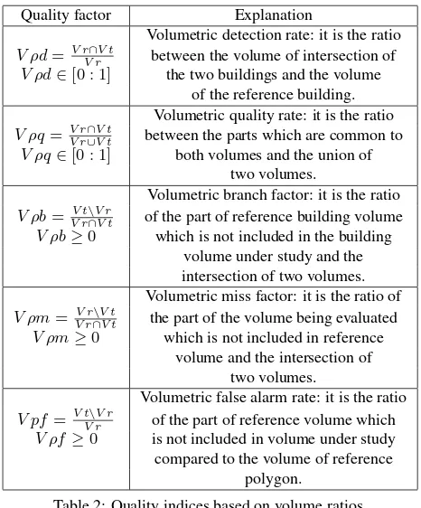
Equations in Table 2 detail the volumetric quality factors. Satis-fying results are reached when the value ofV ρdandV ρqis close to 1, and the three others are close to 0.
Quality factor Explanation
Volumetric detection rate: it is the ratio
V ρd=V r∩V t
V r between the volume of intersection of
V ρd∈[0 : 1] the two buildings and the volume of the reference building. Volumetric quality rate: it is the ratio
V ρq=V r∩V t
V r∪V t between the parts which are common to
V ρq∈[0 : 1] both volumes and the union of two volumes.
Volumetric branch factor: it is the ratio
V ρb= V tV r\∩V rV t of the part of reference building volume
V ρb≥0 which is not included in the building volume under study and the intersection of two volumes. Volumetric miss factor: it is the ratio of
V ρm= V rV r∩\V tV t the part of the volume being evaluated
V ρm≥0 which is not included in reference volume and the intersection of
two volumes.
Volumetric false alarm rate: it is the ratio
V pf=V t\V rV r of the part of reference volume which
V ρf≥0 is not included in volume under study compared to the volume of reference
polygon.
Table 2: Quality indices based on volume ratios.
3 GEOMETRIC COMPUTATIONS
The operation of determining the union and intersection of areas (or volumes) when two models must be compared is a topic of ge-ometric computation. This section describes the algorithms lead-ing to calculate union and intersection of areas/volumes which come into consideration when a model to be assessed is com-pared to a reference model. First of all the areas and volumes of the models under study must be calculated.
3.1 Surface area computation
For the area computation in vector form, we use the formula based on Green’s theorem (O’Rourke, J, 1998) and given in Equa-tion (1).
X and Y are the coordinates of vertices points of the polygon numbered in ascending order.
3.2 Intersection area computation
The operation of determining the intersection area of two vector polygons is performed in two steps: the detection of the points lo-cated inside the polygons and the detection of lines intersections.
Step1: classification of the points located inside the polygons As shown in Figure 2(a), points 3 and 5 are ”inside points”. In Figure 2(b), all points of the red polygon are classified as inside points. Matlab built-in function uses a simple and commonly used technique for point-in-polygon detection, and works as fol-lows. Assuming the polygon is defined bynpoints in an array
P, this algorithm computes the summation of angles between the query point and every pair of points defining each edge of the polygon (i.e. the angle is formed by theP[n]point, query point, andP[n+ 1]). If this summation computes to2π(or near2π
the summation computes to zero (or near zero) then the point is outside the polygon.
Step2: detection of points at the intersection between lines For example, in Figure 2(a), the point of intersection between line (2, 3) and line (5, 6) is a ”point of intersection” to consider, as well as the intersection point of lines (4, 3) and (5, 8). How-ever, the intersection between lines (4, 3) and (6, 7) is not an intersection point to consider. That’s why it must be checked if the intersection point lies on the edges of both polygons. This check is done by computing the distance between the intersection point and the two points of the line. If the maximum of the two distances is shorter than the edge length, the point of intersection belongs to the edge. Then the resulting intersection shape can be calculated based on the coordinates of its vertices (see Equation (1)).
Figure 2: Intersection area calculation for vector polygons in 2D.
3.3 Volume calculation
In order to compute the volume of 3D objects, one has to solve two tasks; firstly determine the convex hull of the given bound-ary, then, calculate the volume of the resulting 3D polyhedron. Convex hull is the boundary of a closed convex surface gener-ated by applying Delaunay triangulation on the corner points. In three dimensions, the convex hull corresponds to a closed polyhe-dron. Convex hull calculation is a hard process in computational geometry (Barber et al., 1996). A large class of algorithms that compute the exact volume of a convex object is based on trian-gulation methods (B¨ueler et al., 1997). The result of convex hull calculation for a gable roof building is shown in Figure 3(a). The convex hull of a set of points in two or three dimensions is given by Matlab built-in function (convhullin 2D orconvhullnin 3D)
as presented in Equation (2). These functions use meshed objects for storing and displaying polyhedra. The faces of such polyhedra are triangles.
[K V] =convhulln(x, y, z); (2)
In 3D, the boundary of the convex hull, K, is represented by a tri-angulated 3D object. It is a set of triangular facets in face-vertex format that is indexed with respect to the point array. Each row of the matrix K represents a triangle. The volume, V, bounded by the 3D convex hull can optionally be returned byconvhulln.
In a first step, the meshed model is computed. It is defined by the input points. The sum of the volumes composing the meshed model equals to the volume of the convex object.
3.4 Intersection volume calculation
The calculation of volume of intersection between two 3D mod-els in vector format is more accurate than in raster format, but also much more complicated. We propose an algorithm allowing to simplify this process. Our method consists of extracting the vertices of 3D intersection volumes. The flowchart in Figure 4 shows the process of intersection volume calculation.
Figure 3: Calculation of convex hull(a) and intersection volume (b).
Figure 4: Flowchart of the method of intersection volume calcu-lation.
The following steps are performed: Step 1: detection of inside points
Extraction of the first group of points is defined by searching about vertices of the reference points located inside the model to assess. This can be done by applying the function”convhulln”
to the points of the model to assess. The points that are inside the reference model are located on the positive side of the plane normals of all of the faces. The result of this process is shown in Figure 3(a) where inside points are in red and outside points in green color.
Step 2: creation of boundary lines and their intersection with planes
The second group of points describing the intersection shape can be determined by calculating the intersection of the lines com-posing the reference model with all planes that are comcom-posing the model to assess. This process can be achieved firstly by sepa-rating the edge lines of each plane of the reference model. Then, the duplicated lines are cancelled in order to avoid repeating the same process. After that, the intersections of all lines with all planes of the model to assess are calculated. In order to check if the resulting point is located on the edge line (and not on the ex-tension of the edge line) and simultaneously belongs to the face of model to assess, two tests should be made. Firstly, we test if the point is placed on the edge line by distance computation as shown in section 3.2. A second test is achieved by looking for the ”points inside a polygon” in 2D (in the frame of the intersected plane), as explained in section 3.2.
Step 3: repetition of steps 1 and 2
4 3D BUILDINGS RECONSTRUCTION
In this paper, three methods for 3D buildings reconstruction are presented.
4.1 Test site and datasets
The study area is located in the city of Strasbourg, France. Dig-ital aerial images from UltraCam-X (4 images) and frame Zeiss LMK (6 images) of the same area were available. Table 3 shows characteristics of the photogrammetric data. Moreover, LiDAR data of the same are has been captured in 2004 (Table 4).
Sensor Ultracam-X Zeiss LMK
Acquisition date 2007 1998
Focal length (mm) 100.500 211.03
Ground Sampling 16 24
Distance (cm)
Pixel size(µm) 7.2 30
Image format 9420 7680
(pixels) by 14430 by 7680
Flying height (m) 2300 1700
Overlap % 65 70
Base (m) 527 556
Table 3: Characteristics of photogrammetric datasets.
LiDAR system TopScan / Optech ALTM 1225
Acquisition date 2004
Flying height(m) 1440
Density of points 1.3 points/m2
Table 4: Characteristics of the LiDAR datasets.
14 ground control points were measured by GNSS. The digital aerial photographs have unknown imaging orientation parame-ters. Using bundle block adjustment, the exterior orientation pa-rameters of the images have been calculated by KLT software. In our application, the camera information was taken from the cali-bration sheet given by the camera owner.
3D reference buildings models have been created based on the photogrammetric processing of images acquired with UltraCam-X stereo-pairs. After relative and absolute orientation of the im-ages, an accuracy of about 16 cm in X,Y and 25 cm in Z can be es-timated for a point digitized in the stereo-pairs. It is satisfactory, considering that the accuracy of the LIDAR point clouds used here is lower (around 30 to 40 cm in X, Y, Z). So, it has been de-cided that the 3D buildings from UltraCam-X stereo-pairs will be used as references for assessing the 3D buildings reconstructed a) from Zeiss LMK stereo-pairs (75 buildings), b) from LiDAR data (8 buildings), and c) from integration of LiDAR and UltraCam-X stereo-pairs (26 buildings). For illustration purposes, only 8 buildings are shown in Figure 7. The reconstructed buildings in the test site have three types of roofs: flat, hip and gable roofs.
4.2 3D models from aerial images
The geometry of objects (roofs, walls, and footprints) are ex-tracted from multiple images. The flowchart of the semi-automatic approach is depicted in Figure 5. The first step of building recon-struction is roof digitizing. Then, the projection of these points onto the ground is done in order to obtain footprints and thus to create the walls. Finally, planes of faces and footprints are cre-ated.
The reconstruction approach is based on the assumption that: (a) every solid object can be described by a decomposition of its boundaries; (b) the walls are vertical and reach either the ground
Figure 5: Flowchart of 3D building modeling from aerial images.
or another surface of the constructed model. The wall faces can be constructed using the outlines of the roofs (no facade details). Therefore it is not necessary to digitize the footprints of the build-ings. In this work, we restrict our study to simple polyhedral models. Figure 7(b) presents 8 of the 75 samples of building models reconstructed in the test site (in yellow colour) as well as the corresponding reference (in red).
4.3 3D models from LiDAR and aerial images
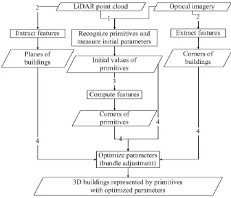
The semi-automatic method proposed by (Zhang et al., 2011) is based on the complementarities of airborne LiDAR and optical imagery (UltraCam-X). It consists of 4 steps (Figure 6).
Firstly, the building is decomposed into several primitives. The primitives parameters are measured manually on LiDAR and aerial imagery, such as length, width, height, orientation and translation of the primitive. These measurements can be used as constraints or initial values in the following optimization procedure. Sec-ondly, features primitives are selected on the imagery. Corners are detected on the optical imagery, and planes are selected in the LiDAR point cloud. These features are used as observations in the following optimization procedure. Thirdly, the algorithm op-timizes primitives parameters by the constraints of LiDAR point cloud and imagery. Based on the type and parameters of primi-tives, the 3D coordinates of the features primiprimi-tives, such as cor-ners, can be calculated. These 3D coordinates will be used as computed values in the next iteration. Finally, 3D building mod-els are produced.
Figure 6: Flowchart of the reconstruction process using LiDAR data and aerial images (Zhang et al., 2011).
This method has been applied to 26 building models of the test site. Figure 7(c) shows 8 of 26 samples of reconstructed buildings (in green) and their reference buildings (in red).
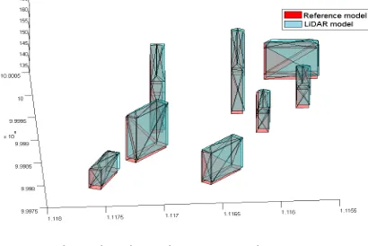
4.4 3D models from LiDAR datasets
(a) Part of the models under study
(b) Models obtained from aerial images (8 of 75 buildings).
(c) Models obtained from aerial images and LiDAR datasets (8 of 26).
(d) Models obtained from LiDAR datasets.
Figure 7: Reference and tested building models.
At first, the point cloud covering the building is segmented to isolate building roofs. Then, a topological graph is constructed
to recognize the shape of the buildings. Finally, once simple roof types are determined, building models are reconstructed with pre-defined models. Outlines of the buildings are first estimated with the minimum area bounding rectangle while the other key ver-tices and segments are obtained through the roof-topology graph. More details are given in (Verma et al., 2008). Figure 7(d) shows the results. The buildings reconstructed from LiDAR datasets are in cyan colour and their reference in red.
5 ASSESSMENT RESULTS
In this section, we assess the 3D vector building models recon-structed previously, by applying the multi-dimensional assess-ment approach suggested in section 2.
5.1 1D assessment
The reference building models are the models reconstructed from UltraCam-X (see section 4.2). Deviations are calculated between centers of gravity of homologous planes that compose the tested and respectively the reference building. Table 5 presents the RMSE results obtained. The models reconstructed from aerial images give better results than the other methods. The models recon-structed from integration of LiDAR and aerial images give high RMSE in Z-direction. Worse results are obtained for models re-constructed with LiDAR data only. The error budget is not only composed of errors due to the reconstruction algorithm, but also of errors coming from the raw data. For instance, low point cloud density and errors due to the georeferencing of the LIDAR and the optical data affect the final results.
Reconstruction RMSE(m)
from X Y Z
Aerial images [75 buildings] 0.21 0.26 0.50 Integration of aerial images and 0.50 0.48 0.94
LiDAR datasets [26 buildings]
LiDAR dataset only [8 buildings] 0.64 0.99 1.00
Table 5: RMSE calculated on gravity centers of homologous planes.
5.2 2D assessment
The statistics of the 2D quality indices calculated for assessing the faces of the building models are summarized in Table 6. For models created from aerial images, the mean values ofρdandρq
are about 0.9 and the other three indices are close to 0. The worse values obtained for the other models are explained by the high RMSE in Y and/or Z-directions (Table 5). This means that the 3D surface of building models extracted from stereo-pairs are close from each other. Also, the models reconstructed from LiDAR or integration of LiDAR and aerial images are less accurate than the models reconstructed from aerial images alone. However, the mean values of quality indices can not be considered alone. In order to evaluate the building reconstruction quality in detail and to analyze the values of the 2D quality factors, one should check the quality indices for each building separately. Moreover, sur-face metrics are affected by the building size. Small buildings generally lead to bad results regarding the 2D quality indices.
Reconstruction ρd ρq ρb ρm ρf
from
Aerial images 0.938 0.891 0.089 0.085 0.062 Images&LiDAR 0.867 0.788 0.177 0.154 0.120
LiDAR only 0.840 0.711 0.219 0.250 0.189
5.3 3D assessment
The results of the quality analysis based on volumetric quality factors are shown in Table 7. The mean values ofV ρdandV ρq
are about 0.9, while the other three indices are close to 0 for 75 models of aerial images. The mean values of volume quality in-dices,V ρdandV ρqare about 0.8. The other three indices are about 0.1 for 8 models created from LiDAR datasets and 26 mod-els of integration of optical and LiDAR datasets. This means that the models reconstructed from aerial images are more accurate than the other models.
Reconstruction V ρd V ρq V ρb V ρm V ρf
from
Aerial images 0.943 0.895 0.063 0.058 0.054 Images&LiDAR 0.875 0.809 0.148 0.102 0.089
LiDAR only 0.885 0.791 0.136 0.136 0.120
Table 7: 3D quality indices.
The 3D assessment provides more information than the 2D as-sessment, because it takes into account the shift which might ex-ist in the third dimension between the two 2D surfaces. This oc-curs for the quality indices obtained for the models reconstructed from the LiDAR dataset. All tests applied on the building models reveal that a systematic error affects the Z coordinates of the LI-DAR data used here. This vertical shift has already been observed in a study where ALS and TLS data were combined (Boulaassal et al., 2011).
6 CONCLUSIONS AND FUTURE WORK
In this paper, three semi-automatic methods for 3D building re-construction in vector format have been mentioned and carried out on the same test site. The quality evaluation of these models has been achieved by applying the proposed multi-dimensional quality assessment approach. This approach considers the accu-racy of the 3D building models based on the comparison of points in 1D, of surfaces in 2D, and of volumes in 3D. 1D assessment gives an overall idea about the reliability of the reconstructed models. 2D assessment checks the superimposition of faces, de-spite its dependency on the size of the polygons to be compared. 3D assessment compares the buildings in 3D through the com-parison of their volumes intersection. It is appropriate for de-tecting the direction of errors (shifts in X, Y, and Z or rotations). This multi-dimensional approach is suitable for 3D building vec-tor models created from aerial images and/or LiDAR datasets. Future researches will focus on the extension of this approach to more complex building models. In this context, it will be focused on the benefits of using raster assessment approaches.
REFERENCES
Barber, C., Dobkin, D. and Huhdanpaa, H., 1996. The Quickhull algorithm for convex hulls. ACM Transactions on Mathematical Software. pp. 469-483.
Boulaassal, H., Landes, T. and Grussenmeyer, P., 2011. Recon-struction of 3D vector models of buildings by combination of ALS, TLS and VLS data. 4th 3D-ARCH International Confer-ence on 3D Virtual Reconstruction and Visualization of Complex Architectures. Trento (Italy), 2-5 March 2011, 6 pages.
B¨ueler, B., Enge, A. and Fukuda, K., 1997. Exact volume com-putation for polytopes : A practical study. Polytopes - Combina-torics and Computation. 18 pages.
Congalton, G. and Kass, G., 2009. Assessing the Accuracy of Re-motely Sensed Data: Principles and Pratices. Taylor and Francis Group LLC. 2nd Ed. 183 pages.
Grussenmeyer, P., Hottier, P. and Abbas, I., 1994. Le contrˆole topographique d’une carte ou d’une base de donn´ees constitu´ees par voie photogramm´etrique. Journal of the French Association of Topography, XYZ . No. 59, pp. 39-45.
Landes, T., Boulaassal, H. and Grussenmeyer, P., 2012a. Quality assessment of geometric facade models reconstructed from TLS data. The Photogrammetric Record. Vol. 27, Issue 138, pp. 137-154.
Landes, T., Grussenmeyer, P., Boulaassal, H. and Mohamed, M., 2012b. Assessment of three-dimensional models derived from LiDAR and TLS data. International Archives of the Photogram-metry, Remote Sensing and Spatial Information Sciences. Vol. XXXIX-B2, Commission II, WG4, pp. 95-100.
McGlone, J. and Shufelt, J., 1994. Projective and object space ge-ometry for monocular building extraction. In: Proceedings Com-puter Vision and Pattern Recognition CVPR ’94, IEEE ComCom-puter Society, Seattle, WA , USA. pp. 54-61.
McKeown, D., Bulwinkle, T., Cochran, S., Harvey, W., McGlone, C. and Shufelt, J., 2000. Performance evaluation for automatic feature extraction. IAPRS International Archives of Photogram-metry and Remote Sensing. Vol. XXXIII, Part B2. Amsterdam 2000. pp. 379 - 394.
Meidow, J. and Schuster, H., 2005. Voxel-based quality evalua-tion of photogrammetric building acquisievalua-tions. In: ISPRS Work-shop on Object Extraction for 3D City Models, Road Databases and Traffic Monitoring (CMRT05), Vol. XXXXVI, Part 3/W24. pp. 117-124.
Mohamed, M. and Grussenmeyer, P., 2011. Plane-based accuracy assessment in photogrammetry: comparison of Rollei medium format and UltraCam-X digital cameras. In: GTC2011 Sympo-sium, Geomatics in the City, Jeddah, Saudia Arabia. 6 pages.
O’Rourke, J, 1998. Computational geometry in C. Cambridge University Press, second edition. 392 pages.
Ragia, L., 2000. A quality model for spatial objects. In: ISPRS Congress, Part B4, Vol. Vol. XXXIII, Amsterdam. pp. 855-862.
Rottensteiner, F. and Briese, C., 2002. A new method for build-ing extraction in urban areas from high-resolution LIDAR data. IAPRSIS. pp.295 301.
Schuster, H. and Weidner, U., 2003. A New Approach Towards Quantitative Quality Evaluation of 3D Building Models. In: IS-PRS com IV, Workshop Challenges in Geospatial Analysis, Inte-gration and Visualization II, Stuttgart, Germany. pp. 156-163.
Tarsha-Kurdi, F., Landes, T. and Grussenmeyer, P., 2008. Ex-tended RANSAC algorithm for automatic detection of building roof planes from Lidar data. The Photogrammetric Journal of Finland. Vol. 21 No.1, pp.97-109.
Verma, V., Kumar, R. and Hsu, S., 2008. 3D building detection and modeling from aerial Lidar data. In: IEEE Computer Soci-ety Conference on Computer Vision and Pattern Recognition. 8 pages.