DIGITAL ELEVATION MODEL APPROXIMATION
FROM STREAM NETWORKS: A REVERSED APPROACH
M. Ghandehari
Department of Surveying and Geomatics Engineering, College of Engineering, University of Tehran, Iran [email protected]
KEY WORDS: Digital Elevation Model, Stream Network, Catchment Area, Stream Order, Skeleton
ABSTRACT:
The delineation of stream networks and catchment areas is one the most common applications of Digital Elevation Models (DEMs). In this article, an innovative reversed approach for the approximation of DEMs from stream networks is presented. As a fundamental preprocessing step, the stream networks are sampled with a set of points. Then, a Delaunay triangulation and Voronoi diagram are used to extract the skeleton (medial axis) of stream networks as an approximation of the catchment areas. The catchment areas contain implicit information that is representative of the terrain, and so the elevation points can be extracted along the catchment area boundaries. Furthermore, we employ the stream orders to enrich the elevation data set. Finally, the elevation points are converted into an elevation grid through a raster interpolation method. While an approximation approach, the results show that the proposed method achieves the desired results.
1. INTRODUCTION
Digital Elevation Models (DEMs) are commonly used in a variety of earth science applications (El-Sheimy et al., 2005; Li et al., 2005). The delineation of stream networks and catchment areas is one the most common applications of DEMs (Martz and Garbrecht, 1993). Assuming that water always flows along the path of the steepest descent, these applications simulate rainfall and extract the cells whose precipitations eventually end up into the same particular point (i.e., the definition of a catchment area). In this article, an innovative reversed approach for the approximation of DEMs from stream networks is presented.
The geometric structure of stream networks can be used to extract topographic information of a terrain, even in the absence of elevation data. The first studies of stream network topology have been conducted by Horton (1945), Strahler (1957), Shreve (1966), and Tokunaga (1978). They used the stream order methods (i.e., a classification of the rank of streams based on a hierarchy of tributaries) to investigate the properties of drainage systems. Nevertheless, stream orders cannot model all the stream characteristics, such as spatial proximity (i.e., distance to connecting streams). In this study, we use stream orders to improve our results. The movement of water over a land surface is determined by the shape of its terrain. Kelley et al. (1988) simulated the terrain using a model of stream erosion. They illustrated that the branching structure of stream networks
contain information about the landscape‟s topographic features.
Since then, several algorithms have been presented by different authors using a fractal model of terrain with rivers (Belhadj and Audibert, 2005; Goodchild and Mark, 1987; Prusinkiewicz and Hammel, 1993; Yokoya et al., 1989). Generally, these algorithms have not become widespread because of complexity and unrealistic models such as flowing of streams in an asymmetric valley. Gold and Snoeyink (2005) proposed a Voronoi-based skeleton extraction method called one-step crust
and skeleton algorithm (Gold and Snoeyink, 2001) for the delineation of catchment areas from stream networks to make a 3-dimensional terrain model. The initial investigations of applying the method to a small dataset show that this method gives a fair approximation of the catchments and terrain model, but it has never been practically evaluated (Gold and Dakowicz, 2005). Furthermore, there are some issues with the one-step crust and skeleton algorithm to be solved in order to be practically used for the catchment area delineation from stream networks. This article aims to examine and expand this investigation. We also attempt to employ the local and global properties of stream networks (e.g., size, proximity, order of streams, etc.) to make an adequate approximation of the DEM.
The best approximation of a catchment area is the region that is closer to a single stream segment (which are the sections naturally defined by branching and confluences of rivers) than to any other (Dillabaugh, 2002; Gold and Dakowicz, 2005; McAllister, 1999). This approximation is obtained using the skeleton, which for a shape is defined as the locus of the centers of circles that are tangent to shape boundary in two or more points, where all such circles are contained in shape. This article investigates the delineation of catchment areas from the skeleton of stream networks.
As a fundamental preprocessing step, the stream networks are first sampled with a set of points. Then, a Delaunay triangulation and Voronoi diagram are used to extract the skeleton of stream networks as an approximation of the catchment areas. Although this idea has been already proposed in the literature, the complexities of the skeleton extraction prevent it from being practically used. A major issue is the appearance of extraneous branches in the skeleton due to perturbations (noise) of the sample points, which must be filtered out in a pre- or post-processing step. This article improves on a Voronoi-based skeleton extraction algorithm by International Archives of the Photogrammetry, Remote Sensing and Spatial Information Sciences, Volume XL-1/W3, 2013
using labeled sample points to automatically avoid extraneous branches.
We extract the skeleton of stream networks as an approximation of the catchment areas. The catchment areas contain implicit information that is representative of the terrain. This information can be extracted and used to approximate the actual terrain. In our approach, even though the elevation information is not available, considering an estimate of slopes for terrain model is meaningful (i.e., the slope on each side of a catchment are often similar), and extracting the elevation points along the catchment area boundaries is possible.
The proximity of catchment boundaries is a local parameter and does not adopt the global shape of a terrain. In other words, the catchment areas can be used to model the relative elevation around each stream. However, more importantly, a global parameter can be derived from the branching structure of stream networks to model the entire terrain. The key idea applied here is the concept of stream orders as a global parameter to enrich the elevation data set.
By using the spatial properties of stream networks, we produce elevation points that are irregularly distributed. According to the U.S Geological Survey (USGS), „a DEM is a digital cartographic representation of the elevation of the land at regularly spaced intervals in x and y directions, using z-values referenced to a common vertical datum‟ (Maune, 2007). To make a DEM, the extracted elevation points are converted to an elevation grid through a raster interpolation approach. Choosing a proper interpolation method is one of the most important issues in DEM generation (Li et al., 2005). There are several methods for raster interpolation, of which we explore three: (i) Inverse Distance Weighting (IDW), (ii) Ordinary Kriging (OK), and (iii) Natural Neighbor (NN). While an approximation approach, the results show that the proposed method achieves the desired results.
2. METHODS
The methods developed in this article employ some geometric structures, including Delaunay triangulation, Voronoi diagram, crust, and skeleton. The definitions of these geometric structures are given in Section 2.1. The skeleton extraction of stream networks is described in Section 2.2. Then, in Section 2.3, the resulting diagram of the skeleton is processed to extract the elevation points. In Section 2.4, we show how stream orders can be used to improve the accuracy of our method. Finally, in Section 2.5, the elevation points are converted into an elevation grid using three different raster interpolation methods (i.e., IDW, OK, and NN).
2.1 Fundamental Geometric Structures
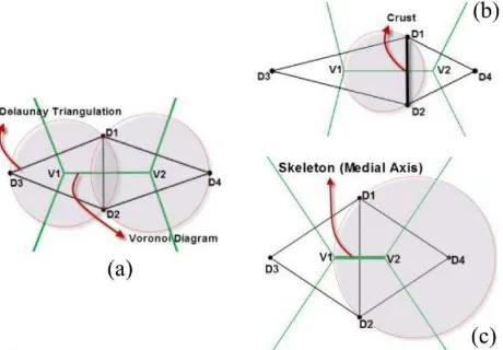
The definitions of Delaunay triangulation, Voronoi diagram, crust, and skeleton are illustrated in Figure 1. The Delaunay triangulation of a set of points in the plane (D1, D2, ... in Figure 1.a) is a triangulation (of this set of points) that satisfies the empty circumcircle property: The circle that passes through the three vertices of each triangle (called circumcircle) does not input point than to any other input point. The Voronoi diagram is the geometric dual of the Delaunay triangulation. This means that the centers of the circumcircles of the Delaunay triangulation are the Voronoi vertices (V1, V2, ... in Figure 1.a); and connecting the adjacent generator points in a Voronoi diagram yields their Delaunay triangulation.
The crust and the skeleton of a set of points can be computed using the associated Delaunay triangulation and Voronoi diagram. Amenta et al. (1998) proposed a Voronoi-based algorithm (called crust algorithm) to reconstruct the boundary of a shape from a set of sample points. Gold and Snoeyink (2001) improved this algorithm so that both the crust and the skeleton are extracted, simultaneously, and they coined the
name “one-step crust and skeleton” for this algorithm. In this algorithm, crust/skeleton is a subset of Delaunay/Voronoi edges. The inclusion of an edge in the structure is determined by a simple inCircle test. Suppose two triangles D1D2D3 and D1D2D4 with a common edge D1D2 whose dual Voronoi edge is V1V2. The InCircle(D1, D2, V1, V2) determines the position of V2 respect to the circle passes through D1, D2 and V1. If V2 is outside the circle, D1D2 belongs to the crust (Figure 1.b); otherwise, if V2 is inside, V1V2 belongs to the skeleton (Figure 1.c).
Figure. 1. Definition of the fundamental geometric structures used by the proposed method: (a) Delaunay triangulation and Voronoi diagram of four sample points D1 to D4; (b) V2 is outside the circle passes through D1, D2 and V1, so D1D2 belongs to the crust; (c) V2 is inside the circle passes through D1, D2 and V1, so V1V2 belongs to the skeleton.
2.2 Skeleton Extraction of Stream Networks
Stream networks can be approximated by sampling. If this sampling is sufficiently dense, the sample points effectively carry the shape information of the stream; i.e., they can be used to reconstruct the original stream and approximate its skeleton.
As mentioned in Section 1, the skeleton is inherently unstable under small perturbations; i.e., it is very sensitive to small changes of the boundary, producing many extraneous branches in the skeleton. Filtering extraneous branches is a common solution to handle this issue; it may be applied as a pre-processing step by simplifying (smoothing) the boundary, or as a post-processing step through pruning, which eliminates the irrelevant branches of the extracted skeleton. However, filtering may alter the topological or geometrical structure of the International Archives of the Photogrammetry, Remote Sensing and Spatial Information Sciences, Volume XL-1/W3, 2013
skeleton. In the following, we propose an improvement to the one-step crust and skeleton algorithm by labelling of the sample points in order to automatically avoid the appearance of extraneous branches in the skeleton.
We observed that the extraneous skeleton edges are the Voronoi edges where the vertices of their dual Delaunay edges lie on the same curve segment, while the main skeleton edges are the Voronoi edges where the vertices of their dual Delaunay edges lie on two different curve segments. Therefore, the main idea of the improved method is to remove all the skeleton edges whose corresponding Delaunay edges lie on the same boundary curve (Ghandehari and Karimipour, 2012; Karimipour and Ghandehari, 2012).
To apply our algorithm, the sample points must be labelled: All junctions are assigned JNC as label. All of the points sampled on each stream segment are assigned the unique label (ID) of that segment during the sampling process.
In practice, labelling is performed manually so that the sample points fairly approximate the curve. This process cannot be fully automated due to the fact that intersection of curve segments (called junctions) must be provided by the user. Fortunately, in case of streams, the junctions of stream networks are well defined (i.e., the intersection of two stream segments), so automatic tools could be deployed for stream network labelling. For a proper sampling, all junctions should be sampled. Then, enough points on each stream segment are sampled so that a fair approximation of the stream shape is provided. We used the
“geometric network” extension of the ArcGIS software to automatically extract the junctions. Then, each stream segment
is sampled using the “feature-to-point” tool, which automatically samples a stream network and assigns the attributes (including the ID) of that stream segment to all of its corresponding sample points.
Filtering in the proposed method is not a pre- or post-processing step, but it is performed simultaneously with the skeleton extraction. To extract the skeleton, we use the one-step crust and skeleton algorithm. The InCircle test is applied on all the Delaunay edges: If the determinant is negative and the corresponding Delaunay vertices have the same labels or one of them is a junction, that Delaunay edge is part of the crust. On the other hand, if the determinant is positive and the corresponding Delaunay vertices have different labels, its dual is added to the skeleton. As illustrated in Figure 2, the extracted skeleton of a stream networks yields a fair approximation of the corresponding catchment areas.
2.3 Extraction of Elevation Points
Even though the elevation information is not available, the slopes on each side of a catchment area are often similar, and so the elevation points can be extracted along the catchment area boundaries.
Figure 2. The skeleton extraction of a stream network yields an approximation of the catchment areas
Our data structure consists of the Delaunay edges that form the crust (i.e., stream), plus the Voronoi edges forming the skeleton (i.e., catchment). Now, we can straightforwardly approximate the elevation at each skeleton edge: the skeleton is at the midpoint between two streams, and hence its elevation is half way between. In other words, the distance between the middle of a skeleton edge and stream is equal to the half of its dual Delaunay edge. So, the elevation points can be obtained automatically from the Delaunay/Voronoi structures (i.e., the crust/skeleton classifications).
2.4 Stream Ordering
The 2-dimensional geometry of stream networks contains implicit information about the topographic characteristics of a landscape. A stream network involves many tributaries, which are merged together and form a hierarchical structure. Assuming that water always flows along the path of steepest descent, the primary branches of the hierarchy are located at the utmost elevation and they make second-class branches at a lower altitude. So, stream orders can identify upstream and downstream locations and reflect the cumulative decrease of altitude in stream branches.
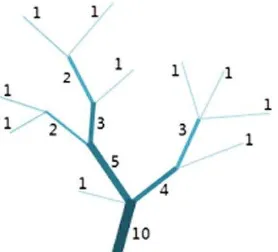
There are several methods for assigning orders to a stream network (e.g., Strahler, Horton, and Shreve). We employ the Shreve method, because in this method the order of each stream is equal to the number of up streams in the network. All streams with no tributaries are assigned an order of one. At the point where two streams intersect, their order are added and assigned to the downslope stream. For example, the intersection of orders 2 and 4 form an order 6 stream. Figure 3 illustrates the ordering of stream networks using the Shreve method.
Figure 3. The ordering of streams based on the Shreve method International Archives of the Photogrammetry, Remote Sensing and Spatial Information Sciences, Volume XL-1/W3, 2013
Stream orders commonly come from raster DEM analysis. But, there are some tools that only use vector stream data and no extra information about slopes and heights is required. Here, we employ the NVS Vector Stream tool developed as an extension of ArcGIS software which simply assigns an order (Srahler or Shreve) to each stream segment based only on a vector stream network (NVisionSolutions, 2013).
Here, we suppose as the stream orders increase, the width and depth of the waterways gradually increase. Now, we can use the stream orders to adjust the altitude of the discussed elevation
Hmean = is the mean elevation of all elevation points Order (p) = the order of point p
Note that the points along the streams get their order from the corresponding stream and the points along the catchment boundaries obtain their orders from the nearest stream. By this modification, the elevation of lower order streams increase more than higher order streams.
2.5 DEM Interpolation
A DEM is often constructed from a set of samples, such that
these samples carry the terrain‟s shape. The samples, in our case, are along the streams and catchment boundaries, which are enough to have a fair approximation of the terrain. In DEM interpolation, we try to produce a gridded surface of elevation data from irregular elevation points using a proper interpolation method. We employ three well-known interpolation methods (i.e., IDW, OK, and NN) that are introduced briefly as follows:
Inverse Distance Weighting (IDW) is one the simplest interpolation methods, whereby values at any unknown points are determined by using a linearly weighted combination (weighted average) of values at nearby known sampled points. Weighting of nearby points is a function of distance; i.e., the closest point to the predicted location would have the most weight (influence) in the interpolation and weights decrease as distance increases from the interpolated points.
Ordinary Kriging (OK) is a geostatistical interpolation method similar to IDW that uses a linear combination of weights at surrounding known points. But, the weights are not only based on the distance, but also on the spatial correlation among the sample points. This means that the spatial arrangement of the samples changes the weights. This property provides an unbiased interpolation with minimum mean square error. There are several types of Kriging, of which we use the ordinary one.
Natural Neighbor (NN) interpolation, also known as
“area stealing”, is a simple method of interpolation.
Choosing neighboring points and computing the weights are the differences between IDW and NN. Finding the appropriate neighbors for interpolation is the strength of this method; the nearest points are chosen using a Voronoi diagram; i.e., only the points whose Voronoi cell has a common boundary with the cell of the unknown point are used. The weights here
are dependent on areas (areas of the neighbors‟ cells) rather than distances.
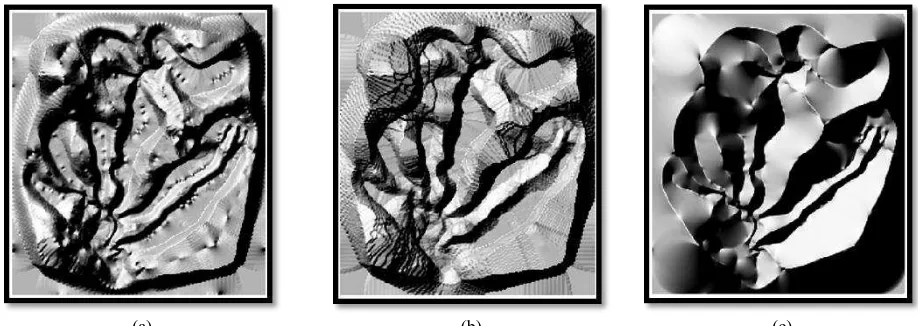
As the accuracy of a DEM depends on the interpolation method used (Hartkamp et al., 1999), choosing a proper interpolation method is an important issue. There is not a single interpolation algorithm that is best for all applications under all conditions (Isaaks and Srivastava, 1989). Figure 4 shows the results of interpolation using IDW, OK, and NN. In Figure 5, for a more effective visualization, we also illustrate the hillshade (a grayscale 3-dimensional representation of the surface in a 2-dimensional perspective view taking the sun's relative position into account) of corresponding DEMs in Figure 4. The outcomes indicate that the NN method is the best and the IDW and OK methods are generally not desirable in our case for several reasons: (1) The strategy of selecting the appropriate neighbors of the point to be interpolated is important and may significantly change the results. NN works properly due to the use of the Voronoi diagram which allows a clear definition of spatial adjacency relationships between the sampled points. (2) The results of most interpolation methods would be similar for enough and well-distributed sample points (Burrough and McDonnell, 1998); however, the selection of interpolation method is more important for unevenly distributed sample points. This is especially true for our case, where elevation points are irregularly distributed. The properties of NN interpolation method make it a good approach for irregularly distributed data; it generates a well-defined set of neighbors (by the use of a Voronoi diagram), and employs a well-behaved weighting function (i.e., the use of stolen areas from the neighboring Voronoi cells). (3) Kriging is usually used for digital elevation modelling; however, it creates a discontinuous DEM (i.e., an abrupt considerable change in elevation) even when the actual terrain is continuous. As illustrated in Figure 5, in NN there is not any concern about discontinuity of the outcomes. (4) High computational requirements are another major shortcoming of Kriging (Burrough and McDonnell, 1998), since it is not efficient for large data sets; However, NN is simply computed from the Voronoi diagram of the sample points. (5) Another problem that can be seen in Figure 5 is the presence of unrealistic undulations in the IDW and OK results. This issue can cause serious problems in some applications such as hydrologic analysis. On the other hand, NN produces a smooth interpolation. (6) Finally, the stream banks (i.e., the "edge" of a stream where the land begins) are well defined in the results of NN method. The cross section of streams in NN shows the same gradual slope that makes an accurate interpolation of stream width. But, the stream width in the other methods unnaturally changes from place to place.
(a) (b) (c) Figure 4. The results of interpolation using: (a) IDW, (b) OK, and (c) NN
(a) (b) (c)
Figure 5. The hillshades of the DEM constructed from (a) IDW, (b) OK, and (c) NN
3. CONCLUSIONS AND FUTURE WORK
Elevation information can be extracted in two ways: explicitly, such as the information in a contour map; or implicitly on the basis of stream network properties. In this article, we have shown that an implicit comprehension of stream networks can lead us to an understanding of topography. The proposed method uses the skeleton and order of stream networks to approximate the DEM. Although our approach is not appropriate for accurate terrain analysis, for non-exact large-scale analysis, it is fast, efficient and yields good results. Additionally, by using well-known data structures in computational geometry like the Delaunay triangulation and the Voronoi diagram, retrieving the original data, constructing topology and improving of the proposed method can all be done easily.
The results showed that the proposed method achieves the desired outcome and provides a fair approximation of the DEM. However, there are a few issues to be investigated in future work: (1) The input of our method is solely the stream networks. We can develop our method by using supplementary data such as ridges, break lines, lakes, islands, etc., to improve the accuracy. (2) The stream order for a stream edge considers a constant altitude for that edge. We are working on more parameters (e.g., flow accumulation) to make a better simulation of water flows in the direction of the steepest downhill gradient. (3) Future research should attempt to introduce new applications for the produced DEM; for example, our DEM can
be useful in hydrological analysis due to the high similarity with hydro-enforced DEMs or in terrain reconstruction for real-time flight simulators.
ACKNOWLEDGMENTS
I acknowledge and greatly appreciate the comments and suggestions from Dr. Farid Karimipour (assistant-professor in the GIS group of the University of Tehran), and Mr Ken Arroyo Ohori (PhD candidate working at the GIS Technology group of the Delft University of Technology).
REFERENCES
Amenta, N., Bern, M.W., Eppstein, D., 1998. The crust and the beta-skeleton: combinatorial curve reconstruction. Graphical models and image processing 60, pp. 125–135. doi: 10.1006/gmip.1998.0465
Belhadj, F., Audibert, P., 2005. Modeling landscapes with ridges and rivers: bottom up approach, Proceedings of the 3rd international conference on Computer graphics and interactive techniques in Australasia and South East Asia. ACM, pp. 447-450. doi: 10.1145/1101389.1101479
Burrough, P.A., McDonnell, R., 1998. Principles of geographical information systems. Oxford university press Oxford. doi: 10.1080/10106048609354060
Dillabaugh, C., 2002. Drainage basin delineation from vector drainage networks. Proceedings Joint International Symposium on Geospatial Theory, Processing and Applications. Ottawa, Ontario, Canada, pp. 8-12.
El-Sheimy, N., Valeo, C., Habib, A., 2005. Digital Terrain Modeling: Acquisition, Manipulation and Applications. Artech House Remote Sensing Library.
Ghandehari, M., Karimipour, F., 2012. Voronoi-based Curve Reconstruction: Issus and Solutions, in: al., B.M.e. (Ed.), The International Conference on Computational Science and Its Applications (ICCSA 2012). Springer-Verlag, Salvador de Bahia, Brazil, pp. 194-207. doi: 10.1007/978-3-642-31075-1_15
Gold, C., Dakowicz, M., 2005. The Crust and Skeleton– Applications in GIS, Proceedings, 2nd. International Symposium on Voronoi Diagrams in Science and Engineering, pp. 33–42.
Gold, C., Snoeyink, J., 2001. A one-step crust and skeleton extraction algorithm. Algorithmica 30, pp. 144–163. doi: 10.1007/s00453-001-0014-x
Goodchild, M.F., Mark, D.M., 1987. The fractal nature of geographic phenomena. Annals of the Association of American Geographers 77, pp. 265-278. doi: 10.1111/j.1467-8306.1987.tb00158.x
Hartkamp, A.D., De Beurs, K., Stein, A., White, J.W., 1999. Interpolation techniques for climate variables. National Resource Group, CIMMYT Mexico, DF.
Horton, R.E., 1945. Erosional development of streams and their drainage basins; hydrophysical approach to quantitative morphology. Geological Society of America Bulletin 56, pp. 275-370. doi: 10.1130/0016-7606(1945)56[275:EDOSAT]2.0. CO;2
Isaaks, E.H., Srivastava, R.M., 1989. Applied geostatistics. Oxford University Press.
Karimipour, F., Delavar, M.R., Frank, A.U., 2010. A Simplex-Based Approach to Implement Dimension Independent Spatial Analyses. Computers & Geosciences 36, pp. 1123-1134. doi: 10.1016/j.cageo.2010.03.002
Karimipour, F., Ghandehari, M., 2012. A Stable Voronoi-based Algorithm for Medial Axis Extraction through Labeling Sample Points, Proceedings of the 9th International Symposium on Voronoi Diagrams in Science and Engineering (ISVD 2012), New Jersey, USA. pp. 109-114.doi: 10.1109/ISVD.2012.20
Kelley, A.D., Malin, M.C., Nielson, G.M., 1988. Terrain simulation using a model of stream erosion. Proceedings of the 15th annual conference on Computer graphics and interactive techniques - SIGGRAPH '88 22, pp. 263-370. doi: 10.1145/378456.378519
Li, Z., Q., Z., Gold, C., 2005. Digital Terrain Modeling: Principles and Methodology. CRC Press, USA. doi: 10.1201/9780203357132
Martz, L.W., Garbrecht, J., 1993. Automated extraction of drainage network and watershed data from digital elevation models. JAWRA Journal of the American Water Resources
Association 29, pp. 901-908. doi: 10.1111/j.1752-1688.1993.tb03250.x
Maune, D.F., 2007. Digital elevation model technologies and applications: The DEM users manual. Asprs Pubns.
McAllister, M., 1999. The Computational Geometry of Hydrology Data in Geographic Information System. Ph.D. Dissertation, University of British Columbia.
NVisionSolutions, 2013. NVS Vector Stream tool.
http://www.nvisionsolutions.com/
Okabe, A., Boots, B., Sugihara, K., Chiu, S.N., 2000. Spatial Tessellations: Concepts and Applications of Voronoi Diagrams (2nd Edition). John Wiley. doi: 10.1002/9780470317013
Prusinkiewicz, P., Hammel, M., 1993. A fractal model of mountains and rivers, Graphics Interface. Canadian information processing society, pp. 174-180.
Shreve, R.L., 1966. Statistical law of stream numbers. The Journal of Geology, 74, pp. 17-37. doi: 10.1086/627137
Strahler, A.N., 1957. Quantitative analysis of watershed geomorphology. Transactions of the American geophysical Union 38, pp. 913-920. doi: 10.1029/TR038i006p00913
Tokunaga, E., 1978. Consideration on the composition of drainage networks and their evolution. Department of Geography, Tokyo Metropolitan University 13, pp.1-27.
Yokoya, N., Yamamoto, K., Funakubo, N., 1989. Fractal-based analysis and interpolation of 3D natural surface shapes and their application to terrain modeling. Computer vision, graphics, and image processing 46, pp. 284-302. doi: 10.1016/0734-189X(89)90034-0