MONITORING CONCEPTS FOR COASTAL AREAS USING LIDAR DATA
A. Schmidt, F. Rottensteiner, U. Soergel
Institute of Photogrammetry and GeoInformation Leibniz University of Hannover
Germany
{alena.schmidt, rottensteiner, soergel}@ipi.uni-hannover.de
KEY WORDS: lidar, digital terrain model, classification, conditional random fields, coast
ABSTRACT:
Coastal areas are characterized by high spatial and temporal variability. In order to detect undesired changes at early stages, enabling rapid countermeasures to mitigate or minimize potential harm or hazard, a recurrent monitoring becomes necessary. In this paper, we focus on two monitoring task: the analysis of morphological changes and the classification and mapping of habitats. Our concepts are solely based on airborne lidar data which provide substantial information in coastal areas. For the first task, we generate a digital terrain model (DTM) from the lidar point cloud and analyse the dynamic of an island by comparing the DTMs of different epochs with a time difference of six years. For the deeper understanding of the habitat composition in coastal areas, we classify the lidar point cloud by a supervised approach based on Conditional Random Fields. From the classified point cloud, water-land-boundaries as well as mussel bed objects are derived afterwards. We evaluate our approaches on two datasets of the German Wadden Sea.
1. INTRODUCTION
The Wadden Sea in the North Sea and the barrier islands are a coastal zone with high spatial and temporal variations. The intertidal zone is located between a section of the coast of north western continental Europe and the Frisian Islands in the southern part of the North Sea. It covers about 10,000 km² and is separated from the North Sea by a barrier island system and ebb-tidal deltas over three quarters of its length. The Wadden Sea consists of tidal mudflats, tidal channels, marshes, and other wetlands; it is a unique ecosystem which is characterized by a high biodiversity. For these reasons the German and the Dutch parts of the Wadden Sea were inscribed on UNESCO's World Heritage List in 2009. The uniqueness of its habitats is accompanied by a high responsibility towards this area and requires a clear understanding of the Wadden Sea’s development.
In the framework of a German research project called Scientific Monitoring Concepts for the German Bight (WIMO, 2013), new approaches for a sustainable monitoring of coastal areas by remote sensing data are investigated. For this purpose, three types of remote sensing data are used: SAR (synthetic aperture radar) data, optical images, and airborne laser scanning data, also called lidar (light detection and ranging). In this paper, we focus on the analysis of lidar data which provide substantial information for two monitoring tasks: change detection of the morphology and the classification of habitats.
Firstly, highly accurate digital terrain models (DTMs) of the Wadden Sea are required for a systematic monitoring of morphological changes. Lidar is a standard method for DTM generation in coastal zones. In comparison to echo sounding systems, lidar is feasible for large areas and delivers dense and accurate data. However, only the eulittoral zone can be covered by standard laser because the near-infrared laser pulses are not able to penetrate water which remains in some tidal channels even during low tide. Thus, gapless DTM modelling usually requires a combination of height data gathered by echo
sounding in the sublittoral zone and airborne lidar systems in the eulittoral zone. In the future the problem of the combination of two different data sources could be overcome to some extent by laser bathymetry. Such modern devices operate with a green laser signal that is capable to penetrate into the water column (e. g. Mandlburger et al., 2011). However, since the accessible depth underneath the water surface depends on turbidity, such technique is better suited for clear waters and not necessarily for the Wadden Sea. In order to detect morphological changes, DTMs of different epochs can be compared. In coastal zones, height differences are caused by tidal flows, storms, strong wind, and human activities like dredging or deepening of channels. For coast protection and the investigation of segmentation and erosion, change detection by airborne lidar becomes substantial.
Secondly, the classification and mapping of habitats in Wadden Sea areas is an important task of marine monitoring. This has been shown to be possible with spectral information from remote sensing image data (Klonus et al., 2012). Due to a lack of spectral features in the monochromatic lidar signal and the common lack of auxiliary aerial photos to support the classification if the flights are performed during night time, the distinction between habitats based on lidar becomes a difficult task. Given these limitations of the data, only habitats characterized by their surface roughness, e.g. mussel beds, can be expected to be distinguished. The detection of these areas is of great interest because the cultivation of mussels in the Wadden Sea and the import of exotic species influences the local morphology and changes the sediment characteristics (Marencic & de Vlas, 2009). The second important classification task is the detection of water areas. Due to the reflection of the near-infrared laser pulses at water surfaces, the elevation measured by standard lidar does not represent the actual terrain level underneath as would be desired. The generation of a DTM thus requires the detection of water surfaces and the use of an additional data source, e. g. sonar, to complete the DTM in these parts.
In this paper, we investigate lidar data acquired over coastal areas in the southeastern part of the North Sea which are used for two substantial tasks in marine monitoring. On the one hand, we analyse two DTMs with a time difference of six years in order to detect morphological changes on an island (Section 2). On the other hand, we classify the lidar point cloud and derive object boundaries in order to contribute to a deeper understanding of the habitats in coastal areas (Section 3).
2. COMPARISON OF DIGITAL TERRAIN MODELS FOR DIFFERENT EPOCHS
For the monitoring of coastal areas based on lidar data, DTMs of different epochs are compared. We use two datasets of an island which were acquired with a time difference of six years. We analyse especially the seaside where larger changes in the topography can be expected.
2.1 Method
The DTMs are calculated by a hierarchic robust interpolation. The approach is based on linear prediction (Kraus & Pfeifer, 1998) and iteratively fits an approximated surface to the point cloud. Each point is weighted dependent on its residuals. Whereas points with positive residuals above the average surface are indicated to belong to objects and receive a low weight, points below the surface are more likely to be ground points and are assigned a high weight. In this way, the surface will be a better and better approximation of the terrain, whereas vegetation and buildings are eliminated from the dataset.
We calculate the DTM in a grid with a width of 1m for each epoch. Afterwards, the differences between both DTMs are determined. We also derive edges from each DTM using a Laplacian of Gaussian filter with σ = 2 pixel. In this way, changes of significant structures in the topography such as break lines can be analysed.
2.2 Test site
The test site is located on the East Frisian Island Juist in the German North Sea. The island has a length of 17 km and is between 500 m and 1 km wide. Because erosion was observed in the west and the north of Juist during the last years, we analyse these parts of the island and choose two different test sites (Fig. 1). In the north we analyse an area of 400 m x 2700 m, the test site in the west has a size of 1050 m x 1150 m.
Figure 1. Orthoimage of the island Juist and the test sites in the north and the west of the island which are outlined.
We compare datasets from two different epochs. The first one was acquired by an ALTM2050 sensor in spring 2004. The second dataset is from spring 2010 using a Harrier 56 sensor.
2.3 Results
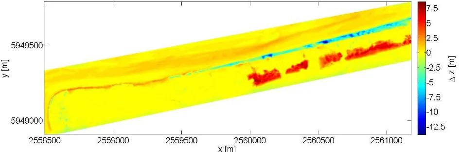
For the monitoring of the topography the DTM of 2004 is subtracted from the DTM of 2010. After six years significant changes in the topography can be observed. Fig. 2 shows the differences of the heights between both epochs in the northern test site. Positive values indicate sedimentation and negative values represent erosion between the epochs. For most of the grid points the differences are low. In the northern test site 86.2 % of all points have changes between -1 m and 1 m (Fig. 3). The mean of the height differences is 0.2 m with a standard deviation of 1.5 m. However, especially in the dunes and at their borders higher differences can be observed. Here, the differences vary between -13.8 m and 8.5 m. Whereas sedimentations occur in the west, the land erodes in the east of this border. The erosion extends over a length of nearly 2 km and is 13.8 m in the maximum. This observation implies that the northern border shifted to the south. Considering the edges derived from the DTM, the amount of the shift can be calculated: it is up to some tens of meters (Fig. 4). To the north of the border, the test site covers coast and sea. Here, the comparison of both DTMs is of limited value due to varying water levels during the data acquisition. In some parts of the dunes significant increases of the heights of up to 8.5 m occur. The changes can be explained by anthropogenic activities in the context of coast protection. Due to continual decrease of sand in this part of the island during the last decades, several supporting measures have been performed. In consequence of a storm tide in the winter of 2006/07, in the south of the dune valleys were recently filled in with sand, which can be verified in the data.
Figure 2. Differences between DTM 2010 and 2004 at the northern border of Juist.
Figure 3. Histogram of the height differences in the northern test site with height variations between -13.8 m and 8.5 m
(values <7m (0.35%) and >7m (0.06%) are not shown)
In the western test site, the height differences between the DTM of 2004 and 2010 are lower. The values vary between -3.9 m and 3.4 m (Fig. 6). The mean of the differences is 0.05 m with a standard deviation of 0.35 m. At seaside, height differences might be caused by different water levels during the acquisition time. This assumption is confirmed by a constant height difference in the tidal channel in the south of the test site. However, the border of the island shows significant topographic changes. At the northern border, sedimentations between 2.0 m and 3.5 m occur over a length of 20 m. The height differences at the western border vary between 1.0 and 2.0 m. Fig. 5 shows the results of the edge detection from both DTMs. In comparison to the northern test site the shift of the border is lower, it is in the range of few meters. Moreover, the edges move predominantly towards seaside between both epochs.
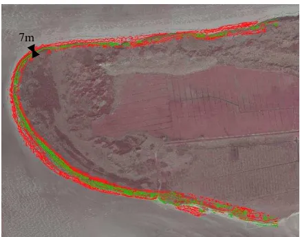
Figure 4. Orthoimage of 2004 and edges derived from the DTM for the dataset of 2004 (green) and 2010 (red) at the northern
border
Figure 5. Edge image with the derived edges for 2004 (green) and 2010 (red) closed to the shoreline
Figure 6. Differences between DTM 2010 and 2004 at the western border of Juist.
3. CLASSIFICATION OF LIDAR DATA
For the mapping of coastal areas, the lidar point cloud is classified in a supervised classification approach (Section 3.1). Each point is classified to one of the three classes water,
mudflat and mussel bed. Afterwards object boundaries are calculated based on 2D binary images derived from the labeled point cloud. We describe the test site and the classification results in Sections 3.2 and 3.3.
3.1 Method
The classification method can be subdivided into three steps: Firstly, lidar features are derived from the point cloud. They are introduced in a classification based on Conditional Random Fields. We classify the data based on the raw lidar point cloud. Then, the labeled 3D point cloud is projected to a 2D label image and object boundaries are calculated.
3.1.1 Feature extraction
We adapted some of the LiDAR features proposed in Chehata et al. (2009) and expand the model by additional features for our classification task (Schmidt et al., 2012a). For each laser pulse, information about 3D coordinates and intensity are available for the backscattered signal. From the point cloud we use the following features:
1) intensity (I)
2) variance of I in a sphere of radius r; 3) point elevation (E);
4) variance of E in a vertical cylinder of radius r; 5) average elevations and their differences for vertical
cylinders with various radii; 6) height above ground;
7) approximated plane: sum of residuals, direction and variance of normal vector;
8) principal curvatures, mean and Gaussian curvature; 9) eigenvalue based features: 3 eigenvalues (λ1,λ2,λ3),
sum (Ʃλ1, λ2,λ3), omnivariance, planarity, anisotropy, sphericity, eigenentropy, scatter (λ1/λ3);
10) point density in a sphere of radius r 7m
The features considering the local point distribution within a sphere or vertical cylinder are computed for multiple scales with radii r = 1, 2, 3, 4, and 5 m. 124 features are determined in total for each point. In order to minimize the complexity of the approach, we do not use all features and identify a representative set for our classification task instead. We analyse the influence of each feature on the classification result by a permutation importance measure (Breiman, 2001). For the importance measurement of a feature, its values are randomly permuted. In this way, feature values with low information for the classification are simulated. Then, the number of correctly classified points before and after permuting the feature values is compared. In case of a high difference between both results, the importance of this feature for the classification task is high. The importance can be determined for each class and for the overall classification. For our classification task, we consider features whose importances are high for the overall classification, and, as the mussel bed detection has proved to be the most challenging task in our previous work (Schmidt et al., 2012), those features which are relevant for the classification of mussel bed. Considering both criteria, we choose the following 14
CRFs provide a flexible framework for many classification tasks and were introduced for image labelling in Kumar & Hebert, 2006. The classification of point clouds based on CRF has been used for instance by Lim & Suter (2009) for the classification of terrestrial laser scanning data. The potential of CRFs for airborne laser scanning data was shown in Shapovalov et al. (2010) (segment-based) and in Niemeyer (2012) (point-based).
CRFs belong to the group of undirected graphical models. The underlying graph G(n, e) consists of nodes n and edges e. Here, the nodes correspond to the lidar points. Each node ni ∊ n is linked to its k nearest neighbours in 2D by edges. We assign a class label from a given set of classes to each lidar point based on the observed data x = [x1,x2,...xm]. The point cloud is classified by finding the optimal label configuration that maximizes the posterior probability P(C|x) of the point labels the exponent are potentials which are explained in more detail at the end of the section. The posterior probability is normalised
P(C|x) the optimal label configuration is estimated.
The potentials of (1) are inferred based on a feature vector hi(x) which contains the lidar features described in Section 3.1.1. There are two potential terms: the associationpotentialAi(x,Ci) and the interaction potentialIi(x,Ci,Cj). They can be expressed by arbitrary classifiers. Following Kumar & Hebert (2006) we use a generalized linear model for both potentials. Then, the
association potentialAi(x,Ci) which indicates the likelihood of a point ni belonging to a class given the observations x can be expressed as
. (2)
In (2) vector wl contains the weights of node features expanded by a quadratic feature mapping function Φ which increase the number of features to 120. The vector wl is determined by a training step. Such a vector is defined for each class l. The dependencies of a node ni from its adjacent node nj is modelled by comparing both node labels and considering the observed data x. We calculated an interaction feature vector µij(x) as the absolute difference of feature vectors of neighbouring nodes ni and nj, µij(x)=|hi(x)-hj(x)|. Analogous to the association
potential, the interaction potential can be modelled being proportional to log P(Ci,Cj| µij(x)). We use a generalized linear model again:
(3)
where vl,k is the weight vector of the interaction features. Such a vector vl,k exists for each combination of classes (l, k). In the training process the optimal values for the weight vectors are derived from training data. The use of exact probabilistic methods for this is computationally intractable. Thus, they are replaced by approximate solutions. Here, we applied the gradient descent optimization method L-BFGS (limited memory Broyden–Fletcher–Goldfarb–Shanno) (Liu & Nocedal, 1989) for the minimization of the objective function f= -log(P (θ| x,C), where the parameter vector θcontains the weight vectors wland vl,k.
3.1.3 Extraction of boundaries
From the classified point cloud, land-water-boundaries and boundaries of mussel beds, respectively, are derived in a post-processing step. First, the labeled 3D point cloud is projected to a 2D label image. Then, binary images for the classes water and
mussel bed are calculated, where nonzero pixels belong to an object and zero pixels to the background. We remove small objects and close small holes using a morphological filtering. From the binary image, the exterior boundaries of the objects and possible holes inside are determined.
3.2 Test site
For the classification of lidar data, we use the dataset of 2010 that was also used for the DTM analysis (Section 2.2). Because we are interested in a mapping of the Wadden Sea for our second monitoring task, we investigate a test site located in the south of the East Frisian Island Norderney. It contains one big tidal channel from north to south and some smaller ones. Although the data were acquired during low tide, water still remains there, especially in the bigger tidal channels, whereas the smaller ones partly dry to muddy channel. In the western part of the tidal channel there are several mussel beds. Whereas the point density is mostly high, the dataset shows the typical
effect of lidar data acquired over water surfaces (and even areas with a small water film): the laser pulses are affected by specular reflection. Depending on the incidence angle the backscatter cannot be recorded by the sensor which leads to gaps in the dataset at the border of the flight strips.
3.3 Results
The outcome of the CRF-classification is a labeled 3D point cloud with three classes: mudflat, water, and mussel bed. The results are depicted in Fig. 7. During the graph generation each point is linked to its two nearest neighbours by an edge. For each point and for each edge we use the 14 features described in Section 3.1 and a quadratic feature space mapping . For the training step we generate a manually labeled reference point cloud including all classes. We use approximately 10 % of the points from the dataset for training.
We get the best results for water surfaces which are classified with correctness and completeness rates of 90.2 % and 95.1 %, respectively (Table 1). Some misclassifications occur near to the mudflat boundaries where local height differences are low. Because of different flight strips in the datasets and thus slightly different water levels caused by tidal effects during the acquisition times, the characteristics of water surfaces vary in the overlap of two strips which leads to some misclassification in these parts. For mudflat the correctness and the completeness rates are 89.3 % and 86.1%, respectively. False positives can be observed especially for points on rough mudflat structures which are incorrectly classified as mussel bed. In comparison to
mudflat and water, the completeness and correctness rates of
mussel bed are lower. Misclassifications are caused by similar feature characteristics of the point cloud on rough mudflat areas or near tidal channels where larger local height differences and deviations of neighbouring points from a local plane occur, too.
In a post-processing step, object boundaries are calculated. By using a morphological filtering, data holes on water surfaces in the classification result are closed and single mudflat points which are depicted as mussel bed are eliminated. The resulting boundaries are shown in Figure 8. Due to not correctly classified water points in the overlapping part of two flight strips, the water surface of the big tidal channel is separated into two objects. Moreover, small holes still remain in the water surfaces. They could be eliminated by stronger smoothing.
class mudflat water mussel bed
correctness 89.3 % 90.2 % 60.1 %
completeness 86.1 % 95.1 % 65.8 %
Table 1. Correctness and completeness rate for the three classes.
4. CONCLUSION
In this paper, we proposed two case studies for monitoring tasks in coastal areas using lidar data: change detection in morphology, and classification of habitats. For the analysis of the morphology, we derived a DTM from the point cloud. By comparing DTMs of different epochs, changes in the terrain were investigated. We analysed data of an island acquired with a time difference of six years. On the borders and in the dunes, significant sedimentations and erosions of several meters can be observed. By comparing the edges derived from the DTMs, the shift of the northern border can be shown. Moreover, the filling of dune valleys as activities in the context of coast protection can be seen in the data.
Figure 7. Reference data (top) and classified point cloud (bottom) with the classes water (blue), mudflat (yellow) and
mussel bed (red). Areas with no return are coloured in white.
Figure 8. Orthoimage and the generated object classes for water
(blue) and mussel bed (red)
For the second task, the lidar point cloud is classified by a supervised classification approach based on Conditional Random Fields. In this way, contextual knowledge is integrated in the classification method. We distinguished three classes namely mudflat, water, and mussel bed. The evaluation of the approach showed good results for the detection of water in lidar data. Only in the overlapping part of different flight strips some misclassifications are caused by tidal effects. The problem could be overcome by extracting features and classifying each flight strip separately. Based on local height differences, curvatures and deviations from a local plane, it is also possible to detect mussel beds in lidar data. However, it has been shown to be a challenging task. False positives occur on rough mudflat parts and due to significant variation of the mussel beds' size. Afterwards, the boundaries of wa ter and mussel bed objects are derived from the lidar point cloud. The water-land-boundaries provide an important input value for terrain modelling. The boundaries of the mussel beds can be used for a habitat mapping of the Wadden Sea.
In the future we intend to investigate the change detection on further test site, e.g. for the determination of the shift of tidal
channels. Moreover, we plan to combine our results with those obtained from optical and SAR images in order to establish a reliable concept for marine monitoring (Schmidt et al., 2012b), and to integrate texture features in the classification process.
5. ACKNOWLEDGEMENT
We would like to thank the Lower Saxon State Department for Waterway, Coastal and Nature Conservation (NLWKN) for providing the LiDAR data.
We used the "Matlab toolbox for probabilistic undirected models", developed by Mark Schmidt. It can be found at http://www.cs.ubc.ca/~schmidtm/Software/UGM.html.
6. REFERENCES
Breiman, L., 2001. Random forests. Machine Learning 45 (1), pp. 5–32.
Chehata, N., Guo, L., Mallet, C., 2009. Airborne lidar feature selection for urban classification using random forests. In: The International Archives of the Photogrammetry, Remote Sensing and Spatial Information Sciences, Vol. XXXVIII, Part3/W8, Paris, France, pp. 207–212.
Klonus, S., Ehlers, M., Schmidt, A., Soergel, U., Adolph, W. and Farke, H., 2012. Change detection in wadden sea areas using RapidEye data, Proceedings of the 32nd Earsel Symposium 2012, Mykonos Island, pp. 18-25
Kraus, K., Pfeifer, N., 1998. Determination of terrain models in wooded areas with airborne laser scanner data. ISPRS Journal of Photogrammetry and Remote Sensing, 53, pp. 193–203
Kumar, S. and Hebert, M., 2006. Discriminative Random Fields. International Journal of Computer Vision, 68(2), pp. 179–201.
Lim, E.H. and Suter, D., 2009. 3d Terrestrial Lidar Classifications with Super-Voxels and Multi-Scale Conditional Random Fields. Computer-Aided Design, 41(10), pp. 701–710.
Liu, D.C. and Nocedal, J., 1989. On the Limited Memory BFGS method for large scale optimization. Mathematical Programming, 45, pp. 503-528.
Mandlburger, G., Pfennigbauer, M., Steinbacher, M. and Pfeifer, N., 2011. Airborne Hydrographic LiDAR Mapping - Potential of a new technique for capturing shallow water bodiesh, In: Modelling and Simulation Society of Australia and New Zealand", pp. 2416 - 2422.
Marencic, H. and de Vlas, J. (Eds), 2009. Wadden Sea - Quality Status Report 2009. Wadden Sea Ecosystem 25. Trilateral Monitoring and Assessment Group, Common Wadden Sea Secretariat, Wilhelmshaven, Germany.
Niemeyer, J., Rottensteiner, F., and Soergel, U., 2012. Conditional random fields for lidar point cloud classification in complex urban areas. In: ISPRS Annals of the Photogrammetry, Remote Sensing and Spatial Information Sciences, I-3. pp. 263-268.
Schmidt, A., Rottensteiner, F., and Soergel, U., 2012a. Classification of airborne laser scanning data in wadden sea areas using conditional random fields. In: International Archives of the Photogrammetry, Remote Sensing and Spatial Information Sciences XXIX-B3. pp. 161-166.
Schmidt, A., Adolph, W., Klonus, S., Ehlers, M., Farke, H., Soergel, U., 2012b. Potential of Airborne Laserscanning Data for Classification of Wadden Sea Areas. Proceedings of the 32th Earsel Symposium, Mykonos Island, pp. 495-502
Schmidt, M., 2012. UGM: A Matlab toolbox for probabilistic undirected graphical models, http://www.di.ens.fr/~mschmidt /Software/UGM.html (2012).
Shapovalov, R., Velizhev, A. and Barinova, O., 2010. Non-associative Markov Networks for 3d Point Cloud Classification. In: Proceedings of the ISPRS Commission III symposium - PCV 2010, International Archives of the Photogrammetry, Remote Sensing and Spatial Information Sciences, 38/Part A, ISPRS, Saint-Mandé, France, pp. 103–108.
Vishwanathan, S. V. N., Schraudolph, N. N., Schmidt, M. W., Murphy, K. P., 2006. Accelerated training of conditional random fields with stochastic gradient methods. In: Proceedings of the 23rd ICML, 2006, pp. 969–976.
WIMO, 2013. Wissenschaftliche Monitoringkonzepte für die Deutsche Bucht (Scientific Monitoring Concepts for the German Bight), http://wimo-nordsee.de (March 4, 2013)