CLASSIFICATION OF PHOTOGRAMMETRIC POINT CLOUDS OF SCAFFOLDS FOR
CONSTRUCTION SITE MONITORING USING SUBSPACE CLUSTERING AND PCA
Y. Xu*, S. Tuttas, L. Heogner, U. Stilla
Photogrammetry and Remote Sensing, Technical University of Munich, Germany - (yusheng.xu, sebastian.tuttas, ludwig.hoegner, stilla)@tum.de
Commission III, WG III/4
KEY WORDS: Scaffolding components, Photogrammetric point clouds, Subspace clustering, PCA, Classification
ABSTRACT:
This paper presents an approach for the classification of photogrammetric point clouds of scaffolding components in a construction site, aiming at making a preparation for the automatic monitoring of construction site by reconstructing an as-built Building Information Model (as-built BIM). The points belonging to tubes and toeboards of scaffolds will be distinguished via subspace clustering process and principal components analysis (PCA) algorithm. The overall workflow includes four essential processing steps. Initially, the spherical support region of each point is selected. In the second step, the normalized cut algorithm based on spectral clustering theory is introduced for the subspace clustering, so as to select suitable subspace clusters of points and avoid outliers. Then, in the third step, the feature of each point is calculated by measuring distances between points and the plane of local reference frame defined by PCA in cluster. Finally, the types of points are distinguished and labelled through a supervised classification method, with random forest algorithm used. The effectiveness and applicability of the proposed steps are investigated in both simulated test data and real scenario. The results obtained by the two experiments reveal that the proposed approaches are qualified to the classification of points belonging to linear shape objects having different shapes of sections. For the tests using synthetic point cloud, the classification accuracy can reach 80%, with the condition contaminated by noise and outliers. For the application in real scenario, our method can also achieve a classification accuracy of better than 63%, without using any information about the normal vector of local surface.
* Corresponding author.
1. INTRODUCTION 1.1 Motivation
In recent years, the efficient and accurate progress monitoring of construction site is becoming more and more popular in the field of project management (Turkan et al., 2012). Good progress monitoring results can help engineers and project supervisors make timely and correct decisions. Classical progress tracking approaches depend highly on field investigations and demand extensive manual work for collection and analysis of acquired survey data and various documents, which not only rely heavily on the personal skills and experiences of managers but also require a lot of time. In the early 2000s, the Architectural Engineering Construction/Facility Management (ACE/FM) industry realized the vital and urgent demand for efficient and accurate construction project progress monitoring (Bosché et al., 2015). After that, the study of automatic construction site monitoring is rapidly developed with the application of 2D imaging, photogrammetry and laser scanning (Turkan et al., 2012). Among all these techniques, the methods based on 3D point clouds are progressively widely used (Tang et al., 2010) because the 3D features and special information in point cloud will facilitate the analysis of monitoring results and fast updating of data.
Building Information Model (BIM), containing the 3D geometry of a building, as well as the schedule information of the construction what extends the 3D to a 4D building model, is
one of the most promising ways of progress monitoring in construction site. However, for the progress monitoring task, the as-planned states of the construction should be compared and adjusted with the as-built state at a certain period (Bosché , 2010). Unlike the as-planned BIM normally generated from 2D plans and blueprints, the as-built BIM is typically created via reverse engineering methods on the basis of measuring results from photogrammetry or laser scanning, for example, dense point clouds (Xu et al., 2015). Nevertheless, the reconstruction of geometric objects from point cloud for as-built BIM is always a challenging task, due to the ambiguous spatial distribution and outliers of the point dataset. Moreover, difficulties on construction sites for the monitoring arise because of possible occlusions during observation, the occurrence of temporary equipment (e.g. scaffolds) and worker or the limited accessibility of acquisition positions. Thus, it is worthwhile to study and develop approaches of reconstructing objects from such point cloud accurately and efficiently.
The scaffolding components, which are common objects appealing in construction site, are always considered to be the disturbing objects when reconstructing as-built BIM, because of the occlusions aroused, similarities with buildings like colour and height and being located very close to the building surfaces. However, since the scaffolds are usually used to assist the construction and the maintenance of building structures, by judging the status of the reconstructed scaffolds, the professionals can also make an appropriate evaluation of the aggregate scheduling for the construction project. Moreover, its
thin, similar and complicated structures, for example, linear shaped boards and tubes with analogous size and scale connected to each other, make it a good experimental dataset for testing potential algorithms and approaches for the reconstruction of as-built BIM.
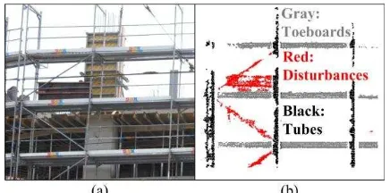
The goal of this research is to automatically classify photogrammetric points of scaffolding components in a construction site. Here, two fundamental elements of scaffolds have been taken into consideration, namely the tube and the toeboard, which are exhibited in Figures 1. For this purpose, we propose a method for the classification of points of scaffolds, with subspace clustering and principal component analysis (PCA) algorithm utilized.
Figure 1. a) Real scene of scaffolds. b) Classification results of toeboards and tubes from generated point cloud.
1.2 Related Work
At the present stage, research work about the classification and recognition of scaffolds components in the environment of construction site using point cloud is scarce. Most of the related work mainly engage in the rebuilding of as-built BIM from point clouds (Pătrăucean et al., 2015; Xiong et al., 2013; Tang et al., 2010) or the comparison between as-built and as-planed BIM for process monitoring (Golparvar-Fard et al., 2011; Tuttas et al., 2014a; Rankohi and Waugh, 2014). On the basis of Scan-vs-BIM system, some applications are also developed using point clouds to trail specified construction objects like Mechanical, Electrical and Plumbing (MEP) components (Bosché et al., 2015) and temporary or secondary objects like shoring, rebar (Turkan et al., 2014).
Beyond these aforementioned work, many research work has been done in the field of recognition and classification of point cloud linking to object of various geometric shapes. Generally, their possible solutions will utilize the geometric feature and statistical information of candidate points with a neighbourhood or support region. For example, 3D shape descriptors such as 3D shape context (3DSC) (Frome et al., 2004), Point feature histograms (PFH) (Rusu et al., 2010) and signature of histogram of orientations (SHOT) (Salti et al. 2014), which count features of local surfaces and spatial distribution of points in neighbourhood as characteristic for point recognition, are commonly used in the matching, classification and reconstruction of point clouds. In our previous work, a preliminary result was achieved (Xu et al., 2015), in which the scaffolding components are detected and reconstructed from a photogrammetric point cloud of a construction site based on projection strategy and 3D shape descriptor. Nevertheless, most of the 3D shape descriptors will depend on the estimation of normal vectors on local surface as a foundation of local reference frame or axis. The accuracy in this case is highly affected by outliers or noise in the dataset.
Another popular way is using the 3D Hough transform, which utilizes the statistical voting procedure in a parameter space and requires no estimation of the normal vectors. For instance, Vosselman et al. (2004) and Borrmann et al. (2011) use the 3D Hough transform for the determination of planar surfaces. Nevertheless, the classification using Hough transform theory is computationally expensive and sensitive to outliers (Maalek et al., 2015). Especially for large datasets, using algorithms based on Hough transform will result in extremely huge computational cost.
The PCA is the eigenvalue decomposition of the covariance matrix of a multivariate data set, which can be used to summarize the variation of the data set with orthogonal axes (Johnson and Wichern, 1992). By applying the PCA, three orthogonal axes can be determined in a three-dimensional point cluster. Some researchers have already used PCA for the classification of point cloud (Rottensteiner et al., 2005; Pu and Vosselman, 2006; Belton and Lichti, 2006; Lari, 2014). However, when the point cluster is contaminated by outliers, the performance of PCA will decline. Thus, in the work of (Maalek et al., 2015), they proposed a classification method of point cloud using robust PCA, in which the PCA is applied to the pre-defined support region of each point. For the points of planar object, the variations in the direction of the surface normal tend to be zero, while, for the points of linear object, all the variations can be summarized in the linear direction.
However, for classifying points of scaffolds, consisting of various linear objects with merely different sections, only calculating the variations by PCA is not sufficient. Moreover, the points in the connection of linear structures will also result in ambiguousness. To that end, a novel approach, which integrates the basic idea of 3D shape descriptor and the advantage of PCA, is proposed to distinguish and classify points of toeboards and tubes from a point cloud of scaffolds. At the beginning, the points in selected spherical support region are segmented via subspace clustering algorithm, in which a normalized-cuts based spectral clustering is adopted, so as to determine the candidate cluster that the points are belonging to. Then, a PCA algorithm is applied to the candidate cluster of points, in order to build a local reference frame (LRF). On the basis of this LRF, all the points in the cluster will be projected to a feature histogram according to the spatial position in LRF. At last, with these feature histograms, all the points are classified by supervised classification methods. The details of the aforementioned stages related to the proposed approach are given in Chapter 2.
1.3 Contribution and Structure
The contribution of this work is twofold. The first one is that we propose a subspace clustering algorithm for point cloud segmentation using normalized-cut based spectral clustering, with spatial distance constraint used. The second one is that we developed a point feature calculation algorithm based PCA and LRF, with no information of normal vector of points requiring, which is motivated by the PCA based points classification method described in (Maalek et al., 2015). Moreover, this work is also an improvement of our former work for the detection and reconstruction of the scaffolding components from a construction site (Xu et al., 2015).
The overall methodology is described in Chapter 2. Firstly, the workflow of all the main steps is briefly depicted in Section 2.1 and the selection of support region is reported in Section 2.2.
Afterwards, Section 2.3 devotes the methods for subspace clustering of points in support region, while the way of calculating point features is described in Section 2.4. Then the methods of supervised classification are given in Section 2.5. In Chapter 3, the experiments are shown, with the introduction of synthetic and real datasets (Section 3.1) and discussion and evaluation of the results (Section 3.2), followed by a conclusion and outlook in Chapter 4.
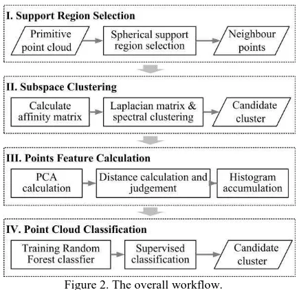
2. METHODOLOGY 2.1 Workflow
The overall workflow for the classification of the scaffolding point cloud can be divided into four essential steps. The first step is to select a support region for each candidate point in the cloud. The whole point cloud has been organised in a k-d tree structure, then a spherical support centring at each feature point is chosen according to a given radius. In the second step, in each spherical support region, a subspace clustering is carried out to segment the points in the support region into several clusters. The candidate cluster in which the feature point is located will be extracted. Subsequently, the points in the candidate cluster will be projected to a feature histogram in accordance with the LRF defined by PCA. Finally, by the use of Random forest algorithm and feature histograms of distances, the linear and planar objects are classified. Figure 2 gives an bunch of candidate points for calculating the distinctive features of the point in the centre of the support region. To simplify the search of points, prior to this selection, the whole point cloud is structured with a k-d tree. Then, the spherical region centred at the feature point is acquired, including points of which the spatial distances between them and the feature point is smaller than the radius of spherical region.
2.3 Subspace Clustering
As for the subspace clustering, we aim to partition points in the support region into subspace clusters, so that the candidate
cluster including the feature point will be determined, because the support region may contain the points of different structures. For example, points in the connection of structure may belong to both vertical and horizontal objects, which is highly likely to result in ambiguousness when applying PCA for defining LRF.
Here, a normalized cut methods based on spectral clustering is conducted (Shi and Malik, 2000). For the 3D points x1, …, xn in the support region X, the similarities W( ji, ) between points
i
x and xj in a similarity matrix W are computed following Equation (1), in which a Gaussian kernel function is used. Considering the spatial distribution of points in isotropic subspace clusters, a strong constraint related to the Euclidean distance between points is introduced. and denote the threshold for this constraint and the parameter of the Gaussian kernel, respectively. The threshold limits the smallest distance between two points belonging to one subspace cluster.
standing for eigenvectors corresponding to k smallest eigenvalues of a normalized L is solved from Equation (4) via the eigenvalue decomposition and normalized Laplacian matrix.
f D f
L (4)
Subsequently, the k-means algorithm is performed on f to partition points into subspace clusters. Note that the number of clusters k is a variable depending on the number of real structural objects in support region. To solve this problem, the variable k is determined by the value maximizing the difference
k
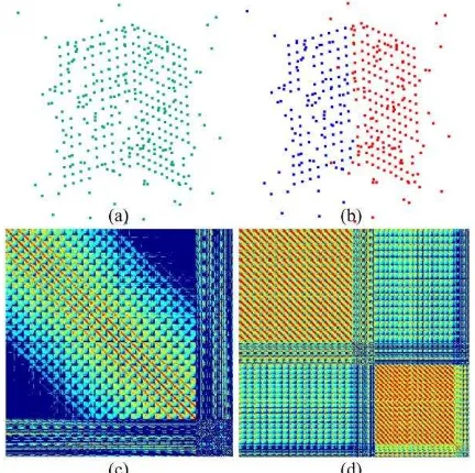
between consecutive eigenvalues k eigengap (Von Luxburg, 2007), which are calculated as shown in Equation (5). results, with the original similarity matrix before subspace clustering and the similarity matrix of two dependent subspaces after clustering illustrated. In these matrixes, the warmer the colour is, the higher the similarity between points is. In this simulated example, a point cluster consisting of two independent structures with contamination of noise is
segmented into subspaces using the aforementioned clustering algorithm. And the dark blue entries mean the similarity is zero, which constrained by .
2.4 Points Feature Calculation
In order to classify point clouds into linear toeboards and tubes, a histogram with three bins accumulating the spatial distance information are calculated as point feature by a LRF. The LRF is a local coordinate frame created and defined in the candidate cluster, attempting to reference all the points in the cluster. Here, PCA is performed to determine the axes of the LRF within the candidate cluster. The origin of LRF is placed at the centroid point, and the Z axis coincides with the linear direction found by PCA.
Figure 3. A simple example of subspace clustering. a) The point cluster contaminated with noises and outliers. b) The subspace clustering results. c) The original similarity matrix. d) The reordered similarity matrix after subspace clustering.
As illustrated in Figure 4, although both the toeboards and tubes of scaffolds have a straight linear shape, the spatial distributions of points in their sections have obvious differences, which are shown up like linear and circular shapes respectively. This can be used to distinguish these two kinds of objects.
Figure 4. Spatial distribution of points in sections of a) toeboard and b) tube.
As shown in Figure 5, for each point P in candidate cluster,
x
d ,dy and dz corresponding to the distances from point to the X-Z plane, Y-Z plane and Z axis are calculated respectively.
Figure 5. a) The local reference frame defined by PCA. b) The distances calculated in local reference frame.
Then, the value of bins of the feature histogram H(i) for i-th point P will be computed following Equation (6). Here, H(i) is
a 1×3 vector, and the value of its elements will be determined by the distances distributed along the Z axis but not around it. Instead, they will be placed close to X axis, so that one bin of histogram will accumulate a relative higher value than others, as shown in Figure 6b. For each feature point, all the points in its candidate cluster will be counted to form its feature histogram.
Figure 6. Two examples of simulated point cloud and accumulated histograms. a) Tube. b) Toeboard.
2.5 Scaffolding Point Cloud Classification
Once the feature histograms of all the points in the whole point datasets are calculated, we use a supervised classification strategy with random forest algorithm to discriminate different kinds of basic elements forming the scaffolds. The feature histograms are employed to train the random forest classifier.
The random forest classifier we utilized (Breiman, 2001) is a combination of N tree-structured classifiers where each decision tree Ti is generated by randomizing vector sampled independently from the input vectors, and each decision tree make a vote consistently for choosing the most popular class to
classify the input vectors (Pal, 2005). The random forest classifier employed in this study consists of using a combination of bins in features histogram at each node to grow a tree. With respect to the training, bagging method is used for each feature combination to generate a training dataset by randomly drawing with replacement N examples, where N is the number of points in each training set (Breiman, 1996). Here, as shown in Figure 7, the training sets are points of two objects, each points is a training sample.
For the classification process, there are two classes
c
1 andc
2 in our case needed to be classified, a sample p(i) will get two confidence degrees after the classification, each confidence degree pc(i) representing the possibility of the sample p(i) belonging to a certain classc
n.As shown in Equation (7), the final output f of the random d forest is the average of the results from all the decision trees.
N i
c
d p i
N f
,..., 1
) ( 1 max
arg (7)
3. EXPERIMENTS
In this study, both the synthetic point cloud dataset and real photogrammetric point cloud of a construction site are utilized in the experiments.
3.1 Synthetic point cloud
The synthetic datasets are simulated point clouds assessing the effectiveness and feasibility of the proposed method, in which a point cloud of artificial structure formed by two kinds of geometric shapes, namely cylinders and cuboids, is created as shown in Figure 9a.
Figure 9. The illustration of synthetic point clouds. a) Original point cloud. b) Point cloud with MN and BG noise.
Aiming at assessing the robustness of the approach, the two kinds of additional noises, the “matching noise” (MN noise) and the “background noise” (BG noise), have also been added to the synthetic point cloud as well. The MN noise attends to mimic the uncertainties of photogrammetric points resulting from the stereo matching process, which is generated by adjusting positions of points in the clouds following Gaussian noise, while the BG noise is to represent outliers in the scene relating to the distractions and mismatches, which is created as additional points randomly distributed in the scene. In the following tests using synthetic datasets, the MN noise points are regarded as inliers being part of the objects. In Fig. 9b, the point cloud adding MN noise and BG noise is given. In the case shown in the figure, the noise level added is 30%. Here, the
noise is assumed to be Gaussian noise, which meets a common normal distribution. The simulated noise level is chosen via the sampling of worst case of real datasets. However, for some cases, such an assumption of noise type and noise level may be inappropriate. Thus, in our future work, we will make further investigations on the optimized selections of noise type and levels in simulations.
3.2 Real point cloud and construction site
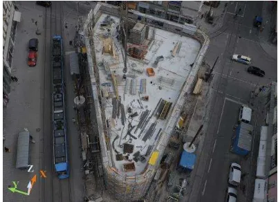
With regard to the real photogrammetric point cloud, we use a construction site as experimental site, with its area on the ground of 2300 m2 and comprising three main façades being triangular in shape. The photogrammetric point clouds are derived by means of structure from motion system and stereo matching method used in (Xu et al., 2015), in which the VSfM Software (Wu, 2013) and LibTSgm (Rothermel et. al., 2012) are used. In Figure 10, an example image taken over the investigated construction site is shown.
Figure 10. Imagery of the construction site taken from the crane.
The dense point clouds created from the images are illustrated in Figure 11. There are 81 images used and 33 million points generated. The detailed camera positions can be found in our former work (Tuttas et al., 2014b). The coordinate system of the point data is perpendicular to the earth ground. As seen from Figure 10, the point clouds contain a lot of noise and outliers and many disturbing objects nearby the main body of the building.
Figure 11. The dense point cloud generated from the images.
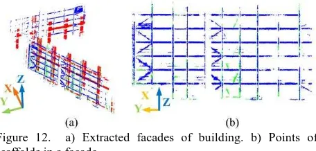
The point cloud of scaffolding components is detected and extracted using the method described in (Xu et al., 2015), which is shown in Figures 12a and 12b. Here, the red points represent the points of the building surface, while the blue and green points stand for the points of scaffolding components.
Figure 12. a) Extracted facades of building. b) Points of scaffolds in a facade.
4. RESULTS 4.1 Results using synthetic point cloud
In Figure 13, classification results using synthetic point clouds of two different noise levels are given. The point clouds have been classified into three categories, namely the points of tubes coloured with blue, the points of toeboards coloured with red and the points of scatters in green. Here, scatters denote noises and outliers, and for the synthetic point cloud used in Figure 13a, there is no scatter (i.e. noise), while for the synthetic point cloud utilized in Figure 13b, it has a noise level of 30%. It can be seen from Figure 13a that the points belonging to different objects are clearly distinguished. According to the confusion matrix in Table 1, the accuracy of the result for tubes is around 94%., but the accuracy of the result for scatters seems to be worse. This is because actually there is no scatter points in the synthetic point cloud used in Figure 13a and there is only very few points being wrongly classified as scatters. Whereas for the result shown in Figure 13b, in the connection area of two objects, many points are misclassified. In Table 2, we give a confusion matrix of the result, with accuracy of classification dropped to around 80%. One possible explanation to this misclassification phenomenon in connection parts is that the subspace clustering may not find correct candidate cluster for the feature point, so that the estimation of LRF has biases.
Figure 13. Classification results of synthetic point cloud. (a) Without noise. (b) With a noise level of 30%.
Moreover, the outliers are also a crucial factor having negative effects on the accumulation of the feature histograms. As seen from Table 2, more than 10% of the points of the tubes and toeboards are wrongly classified as scatter. Thus, in our future work, we may introduce some filtering algorithm while the subspace clustering, in order to eliminate such detrimental influence. It is also noteworthy that the last column of Table 1 is all zero. This is because the first simulated dataset having no points of scatters, so that the predicted true value of scatters should be zeros, and the classified results of scatters are all wrong ones.
Category Tube Toeboard Scatter
Tube 94.55% 5.45% 0%
Toeboard 0.58% 99.42% 0%
Scatter 53.66% 46.34% 0%
Table 1. Confusion matrix of synthetic point cloud result without noise.
Category Tube Toeboard Scatter
Tube 83.57% 2.86% 13.57%
Toeboard 6.59% 80.39% 13.02%
Scatter 24.56% 17.98% 57.46%
Table 2. Confusion matrix of synthetic point cloud result with noise level of 30%.
4.2 Results using real point cloud
The subspace clustering algorithm described in Section 2.3 is performed on the points in one spherical support region, and some intermediate results of clustering are illustrated in Figure 14. It can be seen from Figure 14a that, the feature point centred in the support region is located in the connection position of one tube and two toeboards. The segmented four subspace clusters are shown by different colours. The red one, in which the feature point is situated, is chosen as candidate cluster for calculating the feature histogram. Note that in this support region, there should be five isotropous subspace clusters, but in the clustering result, we can obtain only four segments. One cluster is not recognized. Try to analyse the reason, in Figure 14b, we give an illustration of the similarity matrix according to the clustering result, which is calculated using the clustering results obtained. From the similarity matrix, it can be found that the boundaries between bright square matrixes of numbers II, III and IV which are ambiguous corresponding to the subspace clusters, reveal the sensitivity of eigenvector decomposition when dealing with real noisy point data.
Figure 14. Subspace clustering result in one support region. (a) Subspace clusters. (b) Reordered similarity matrix.
In Figure 15, feature histograms of example points in each cluster shown in Figure 14 are given. As seen from the obtained histograms, it is clear that, for clusters I and II with linear cuboid shape the values of bins in their histograms show apparent falls between bin 1 and bins 2 and 3. Whereas for cluster IV linking to cylindrical shape, the changing of bin values in the histogram shows a slight tendency, which is quite different from those of clusters I and II. As for the cluster III, the one representing points of strut bar with cylindrical shape but contaminated with planar distributed outliers, the bins of its histogram show an intermediate variation trend. This may result in ambiguousness in the classification process using random forest algorithm.
Figure 15. Feature histograms for one point in different clusters. (a) Cluster I. (b) Cluster II. (c) Cluster III. (b) Cluster IV.
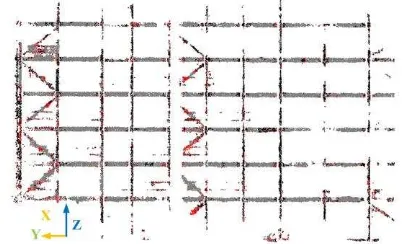
In Figure 16, a final classification result of real scaffolding components in one building facade is displayed, in which all the points are classified into three categories, namely points of toeboard, tube and scatter. Here, the points of scatters may include all the points that do not belong to toeboards or tubes. A confusion matrix is given in Table 3 as well. In Table 3, the rows represent the predicted results, namely the ground truth, while the columns stand for the classification results. The reference data used as ground truth for evaluation is manually segmented.
Figure 16. Classification result of real photogrammetric point cloud.
As shown in Figure 16, most of the points belonging to the toeboard are successfully recognized and classified. However, there are also lots of points belonging to scatters wrongly classified to the category of toeboard, which are in fact points of oblique strut bars but contaminated with outliers. The classification accuracy of points belonging to toeboard is around 70%. It is noteworthy that many points in the connection parts of tubes and toeboards are obviously wrongly classified. For example, in the result of points of tube, more than 25% of points are wrongly recognized as that of toeboards, and only approximately 63% points are correctly classified. One possible origin for such errors is likely to be the error in subspace clustering. If the feature point is improperly clustered, the corresponding LRF will be defined incorrectly, which will lead to a totally wrong accumulation of the histogram. In addition, the outliers and noises existing in the dataset will also have a negative influence on the accumulation of bins in the histogram. For instance, the uncertainties of points generated via stereo matching may deform the surface points of cylindrical objects and make it like a planar surface, which will create a wrong histogram. All these mentioned drawbacks are needed to be taken into consideration in future improvements of this approach.
Category Tube Toeboard Scatter
Tube 63.03% 26.17% 10.79%
Toeboard 12.61% 70.25% 17.14%
Scatter 34.95% 30.47% 34.58%
Table 3. Confusion matrix of real point cloud result.
5. CONCLUSIONS AND FUTURE WORK In this work, an approach, which is a combination of the feature expression idea of 3D shape descriptor and the frame orientation using principal components, is introduced, for the purpose of recognizing and classifying the points of scaffolding components in a construction site. By the use of involved subspace clustering algorithms and PCA method, the points are classified, with both synthetic and real point cloud used. The results indicate that the proposed approaches are competent to the classification of points belonging to two basic scaffolding elements: tubes and toeboards. For the test using synthetic point cloud, the classification accuracy is about 80% in our experiment, with the condition contaminated by noise and outliers. For the test in real scenario, our method can also achieve a classification accuracy of better than 63%, without using any information about the normal vector of local surface. However, there are also some drawbacks, such as the ambiguousness in the partition of subspace clusters and the sensitivity to noise and outliers when accumulating the feature histograms. And also, currently, the proposed methods cannot handle all types of scaffolds in usage, such as scaffolds involving different types of objects.
In future, our work will emphasize on the robust subspace clustering and PCA calculation of points, which can largely limit the performance of the final classification. The performance evaluation should be further investigated. Furthermore, more classifiers will also be taken into consideration, so that our work can be elaborately compared with previous work.
REFERENCES
Belton, D. and Lichti, D., 2006. Classification and segmentation of terrestrial lasers canner point clouds using local variance information. International Archives of Photogrammetry, Remote Sensing and Spatial Information Sciences, Dresden, Germany, 36 (Part 5), pp. 44-49.
Borrmann, D., Elseberg, J., Lingemann, K. and Nüchter, A., 2011. The 3D Hough Transform for plane detection in point clouds: A review and a new accumulator design. 3D Research, 2(2), pp. 1-13.
Bosché, F., 2010. Automated recognition of 3d cad model objects in laser scans and calculation of as-built dimensions for dimensional compliance control in construction. Advanced Engineering Informatics, 24(1), pp. 107–118.
Bosché, F., Ahmed, M., Turkan, Y., Haas, C. T. and Haas, R., 2015. The value of integrating Scan-to-BIM and Scan-vs-BIM techniques for construction monitoring using laser scanning and BIM: The case of cylindrical MEP components. Automation in Construction, 49, pp. 201-213.
Breiman, L., 1996. Bagging predictors. Machine Learning , 24(2), pp. 123-140.
Breiman, L., 2001. Random forests. Machine learning, 45(1), pp. 5-32.
Frome, A., Huber, D., Kolluri, R., Bülow, T. and Malik, J., 2004. Recognizing objects in range data using regional point descriptors. In: Computer Vision-ECCV 2004, Springer Berlin Heidelberg, pp. 224-237.
Golparvar-Fard, M., Peña-Mora, F. and Savarese, S., 2011. Monitoring changes of 3D building elements from unordered photo collections. In: ICCV Workshop 2011, Barcelona, Spain, pp. 249-256.
Johnson, R. A. and Wichern, D. W., 1992. Applied multivariate statistical analysis. Englewood Cliffs, NJ: Prentice Hall, 4.
Lari, Z., 2014. Adaptive Processing of Laser Scanning Data and Texturing of the Segmentation Outcome. Ph.D. Thesis University of Calgary.
Maalek, R., Lichti, D. D. and Ruwanpura, J., 2015. Robust Classification and Segmentation of Planar and Linear Features for Construction Site Progress Monitoring and Structural Dimension Compliance Control. ISPRS Annals of Photogrammetry, Remote Sensing and Spatial Information Sciences, 1, pp. 129-136.
Pal, M., 2005. Random forest classifier for remote sensing classification. International Journal of Remote Sensing, 26(1), pp. 217-222.
Pătrăucean, V., Armeni, I., Nahangi, M., Yeung, J., Brilakis, I. and Haas, C., 2015. State of research in automatic as-built modelling. Advanced Engineering Informatics. 29(2), pp. 162-171
Pu, S. and Vosselman, G., 2006. Automatic extraction of building features from terrestrial laser scanning. International Archives of Photogrammetry, Remote Sensing and Spatial Information Sciences, Dresden, Germany, 36 (5), pp. 25-27.
Rankohi, S. and Waugh, L., 2014. Image-based modeling approaches for projects status comparison. In: CSCE 2014 General Conference, 30, pp.1-10.
Rothermel, M., Wenzel, K., Fritsch, D. and Haala, N., 2012. SURE: Photogrammetric Surface Reconstruction from Imagery. In: LC3D Workshop, Berlin, 8.
Rottensteiner, F., Trinder, J., Clode, S. and Kubik, K. 2005. Using the Dempster Shafer method for the fusion of LIDAR data and multispectral images for building detection. Information Fusion, 6 (4), pp. 283-300.
Rusu, R. B., 2010. Semantic 3d object maps for everyday manipulation in human living environments. KI-Künstliche Intelligenz, 24(4), pp. 345-348.
Salti, S., Tombari, F. and Di Stefano, L., 2014. SHOT: unique signatures of histograms for surface and texture description. Computer Vision and Image Understanding, 125, pp. 251-264.
Shi, J. and Malik, J., 2000. Normalized cuts and image segmentation. IEEE Transactions on Pattern Analysis and Machine Intelligence, 22(8), pp. 888-905.
Tang, P., Huber, D., Akinci, B., Lipman, R. and Lytle, A., 2010. Automatic reconstruction of as-built building information models from laser-scanned point clouds: A review of related techniques. Automation in construction, 19(7), pp. 829-843.
Turkan, Y., Bosché, F., Haas, C. T. and Haas, R., 2012. Automated progress tracking using 4d schedule and 3d sensing technologies. Automation in Construction, 22, pp. 414–421.
Turkan, Y., Bosché, F., Haas, C. T. and Haas, R., 2014. Tracking of secondary and temporary objects in structural concrete work. Construction Innovation: Information, Process, Management, 14(2), pp. 145–167.
Tuttas, S., Braun, A., Borrmann, A. and Stilla, U., 2014a. Comparison of photogrammetric point clouds with bim building elements for construction progress monitoring. In: International Archives of Photogrammetry, Remote Sensing and Spatial Information Sciences Vol. XL-3, pp. 341–345.
Tuttas, S., Braun, A., Borrmann, A. and Stilla, U., 2014b. Konzept zur automatischen Baufortschrittskontrolle durch Integration eines Building Information Models und photogrammetrisch erzeugten Punktwolken. In: DGPF Tagungsband, 23, pp. 363-372.
Von Luxburg, U., 2007. A tutorial on spectral clustering. Statistics and computing, 17(4), pp. 395-416.
Vosselman, G., Gorte, B., Sithole, G. and Rabbani, T., 2004. Recognizing structure in laser scanner point clouds. In: International Archives of Photogrammetry, Remote Sensing and Spatial Information Sciences, 46 (8), pp. 33-38.
Wu, C., 2013. Towards Linear-Time Incremental Structure from Motion. In: 2013 International Conference on 3D Vision, Seattle, WA, pp. 127-134.
Xiong, X., Adan, A., Akinci, B. and Huber, D., 2013. Automatic creation of semantically rich 3D building models from laser scanner data. Automation in Construction, 31, pp. 325-337.