Optimal extraction of Tropospheric Ozone Column by simultaneous use of OMI and TES
data and the surface temperature
Mohammad Reza Mobasheri1, Hamid Shirazi2
1. Department of Remote Sensing Engineering, KNToosi University of Technology ([email protected]) (corresponding author)
2. MSc. Student, Khavaran Institute of Higher-education (KHI), Mashhad, Iran ([email protected])
KEY WORDS: Tropospheric Ozone, OMI, TES, Remote Sensing, Surface Temperature, Nitrogen Dioxide, Radiative Flux
Abstract:
This article aims to increase the accuracy of Ozone data from tropospheric column (TOC) of the OMI and TES satellite instruments. To validate the estimated amount of satellite data, Ozonesonde data is used. The vertical resolution in both instruments in the tropospheric atmosphere decreases so that the degree of freedom signals (DOFS) on the average for TES is reduced to 2 and for OMI is reduced to1. But this decline in accuracy in estimation of tropospheric ozone is more obvious in urban areas so that estimated ozone in both instruments alone in non-urban areas show a high correlation with Ozonesonde. But in urban areas this correlation is significantly reduced, due to the ozone pre-structures and consequently an increase on surface-level ozone in urban areas. In order to improve the accuracy of satellite data, the average tropospheric ozone data from the two instruments were used. The aim is to increase the vertical resolution of ozone profile and the results clearly indicate an increase in correlations, but nevertheless the satellite data have a positive bias towards the earth data. To reduce the bias, with the solar flux and nitrogen dioxide values and surface temperatures are calculated as factors of ozone production on the earth’s surface and formation of mathematical equations based on coefficients for each of the mentioned values and multiplication of these coefficients by satellite data and repeated comparison with the values of Ozonesonde, the results showed that bias in urban areas is greatly reduced.
1-Introduction
Due to the harmful effects of ozone on human health and agricultural production, the estimation of tropospheric ozone vertical profiles to better understand the role of this gas in the different layers of the atmosphere is very important. For example, ozone in the upper troposphere as a greenhouse gas in the middle troposphere as the oxidizing and also near the Earth's surface is known as the main component of photochemical smog (Jacob, et al., 1999). Therefore, given the limitations of the earth-based equipment to estimate tropospheric ozone vertical profiles, the use of satellite equipment in the last five decades has been of main concerns. And the first efforts in this direction is in 1963 and the launch of COSMOS-45 satellite along with UVSP instrument. Thereafter, several satellites, including NIMBUS series NOAA1 and AURA were put in the
1- National Oceanic and Atmospheric Administration
2-Ozone Monitoring Instrument
3- Tropospheric Emission Spectrometer
orbit. The AURA satellite launched in July 2004 into a polar, sunsynchronous orbit to study atmospheric components and their variations with 4 instruments at an altitude of approximately 705 km and with a16-day repetition period and with an ascending equator crossing time of ∼13:45. The two instruments, OMI2 and TES3, were on the AURA platform, and almost simultaneously produce data including the amounts of atmospheric components, such as ozone, nitrogen dioxide and water vapor. The basis for extracting ozone at both instruments is optimal estimation method (Rodgers, 2000).
2- Satellite Measurements and Ozonesonde
atmospheric emission in the thermal infrared (TIR) at the 9.6-m ozone absorption band (Chance, et al., 1997).
2-1 The Measurement of Ultraviolet Band
The observations on the ozone absorption bands in the ultraviolet part of electromagnetic spectrum in range of 290 to 320 nm atmospheric radiation, with the help of spectrometer of moderate resolution and signal ratio to high noise provides a lot of data about tropospheric ozone profiles that the accuracy and precision of this information in the tropospheric part of atmosphere is directly related to the influence of these wavelengths in the atmosphere. The amount of influence of these wavelengths is related to the amount of their absorption at different temperatures and also depending on the Rayleigh scattering in the atmosphere (Chance, et al., 1997). The information of the wavelengths shorter than 290 nm is more related to upper stratosphere. The wavelengths longer than 320 nm, also, (although the penetrating the tropospheric part of the atmosphere) due to the decreased sensitivity to ozone hardly give information from the tropospheric part of the atmosphere (Spurr, et al., 2001). OMI is a nadir-viewing imaging spectrograph that takes measurements of the backscattered solar
radiation from the Earth’s atmosphere and surface in the
ultraviolet and visible region in the wavelengths of 270-500 nm with spectral resolution from 0.42 to 0.63 nm and with 114 degree field of view (the swath-width equivalent to 2,600 kilometers) measure with the help of a row of 30 of the detectors. The ozone profiles are estimated with the help of observations in the UV-1 band and in the spectral range of 264 to 311 nm. And the instrument according to the geometry of observations is able of daily global coverage of the data provided. This instrument does not have a separate product as tropospheric ozone profile. Therefore, in this study, we used the total ozone column profiles of the instrument with the spatial resolution of approximately 50 × 50 km (in the center of swath-width of imaging, at the equator). The third edition of the data, the ozone column, from the earth’s level to a height of about 60 kilometers, is divided into 18 layers from which 5-6 layers are in the troposphere part of the atmosphere. To estimate the ozone profile, the OMI instrument uses optimal estimation method. The basis of this method is to minimize the difference between observed and simulated back-scattered radiances with the help of radiance transfer models. The models with the introduction of primary ozone's profiles and ozone absorption coefficient at different pressures and temperatures, and also the laws of absorption and distribution of the relay simulated the back-scattered radiances received by the instruments. It is worth mentioning that the initial profiles introduced to the algorithms provided of networks of Ozonesonde data to a height of about 30 km of the atmosphere and the information related to higher elevations resulted from the SAGE1 instrument data (McPeters, et al., 2007).
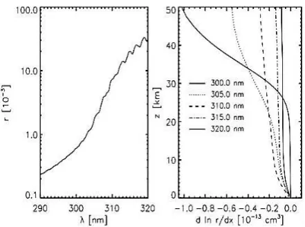
Figure 1 (left window) shows the simulated amount of back-scattered radiance to the instrument, at an angle of 60 degrees Solar Zenith and the Zenith view angle of 10 degrees, and with the assumption of being the Lamberti level and its%5 Albedo (Landgraf & Hasekamp, 2007). In this figure, in the shorter
1-Stratospheric Aerosol and Gas Experiment
wavelengths, because of much absorption of ozone the amount of radiances toward the instrument are low, but in higher wavelengths because of the reduction of ozone absorption, back- scattered radiances increase. Also, Figure 1 (the right window) shows the sensitivity to different wavelengths of UV in relation to the vertical distribution of ozone in the atmosphere. In this figure, the vertical distribution of ozone and temperature changes is based on American standard atmospheric model. As it turns out the shorter wavelengths due to greater sensitivity to ozone, high-altitude of atmosphere are affected with the absorption and scattering and return toward the instrument, and contains information from the stratosphere part of the atmosphere. But the longer wavelengths because of penetrating more in the lower layers of atmosphere contain more information from this section. Nevertheless, by increasing temperature and pressure and changing the absorption coefficient of ozone near the Earth's surface, longer wavelengths show much less sensitivity to the ozone existing in this part of the atmosphere. As seen in the right window, at altitudes less than 5 km, the sensitivity to ozone of all wavelengths under the study is very trivial.
Figure 1- (left side) back-scattered radiances to the instrument in a 290 to 320 nm range (right side)
2-2 Measurements of Thermal Band
Figure 2 - The radiation spectrum in the ozone absorption band using the standard profile of America temperature and level of emissivity of 0.97 and Zenith satellite visibility
angle of 10 °
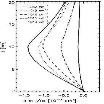
Therefore, the radiation received by the instrument from different altitudes of ozone dependent on vertical distribution of ozone in the line of sight of measurement instrument. In general, it is concluded that radiation resulting from its upper atmosphere layer include the thermal radiation of the layer itself and also the weak signals received from the lower layers. Figure 3 shows the sensitivity to measurements in the thermal infrared band in relation to changes in density of vertical ozone at altitudes of less than 20 kilometers (Landgraf & Hasekamp, 2007).
Figure 3- The sensitivity of thermal infrared radiation to the vertical distribution of ozone using American standard atmospheric
model
According to the above mentioned information, the calculation of radiation received by the instrument from each of the layers of the atmosphere is to be possible with the help of Equation 1:
��
��= [� � − � ] −�� �∆�
�� (1)
In this equation, B is the irradiance spectrum of a black body
along the line of instrument vision, and T is the temperature of each of the layers of the atmosphere used in the standard model.
I0is the radiation from the lowest layer, and also x∂ is the ozone
density in each layer. Also, Δτ is the difference of the two layers consecutive optical depth and τs is the optical depth in the diagonal line of sight from the highest to the lowest layer. TES instrument is a thermal spectrometer whose observations are with spectral resolution of about 0.5 nm in nadir-viewing and 0.1 nm in diagonal cross in the spectral range from 3.2 to 15.4
m. Having two observational cases in this instrument is necessary because the densities of some atmospheric components such as nitrogen oxides in the atmosphere are minimal and the diagonal viewing provided for the observation of long distances results in improvement in measurements of atmospheric components as such. The ozone profiles of TES from the observations at 9.6 m ozone absorption band derived in the spectral range from 9.14 to 9.88 m (Nassar, et al., 2008). Standard data of TES in nadir-viewing case include 16 orbits per 26 hours with spatial resolution of 8.4 km (every 182 km, one profile) in the derived rout. The global coverage for this type of data is obtained every 16 days (Beer, 2006). Also, the instrument data third- processing as networking within 2 degrees latitude and 4 degrees of longitude distances (From the outcome of the interpolation of profiles of second-order process) are available on a daily basis. The data used in this study is the fourth edition includes profiles of ozone from the earth to 4.6416 hpa pressure in the layer of 15 of the atmosphere that the average height of each layer in the troposphere is about 2.4 km. The estimate of the ozone amount in the instrument is also based on radiation transfer models and coefficients related to radiation ozone molecules at various temperatures and pressures. In addition, initial profiles of ozone for TES algorithms are derived from meteorological data MOZART1. These profiles are derived directly from the monthly average values of MOZART (Park, et al., 2004)
2-3. Data Ozonesonde
In this article, the data is used from the network of permanent stations ESRL2 in the Northern Hemisphere, between latitudes 19 to 42 degrees. Usually at the beginning of each week a balloon is sent to collect information on all stations in the network from the profiles of ozone, temperature, humidity and pressure of the Earth's surface up to an altitude of about 32 kilometers of the atmosphere. The profiles are interpolated based on the latitudes of 100 meters in the atmosphere.
3- Optimal Estimation
In order to verify the accuracy of satellite measurements of profiles, averaging kernel can be used per instrument. The averaging kernel using instrument characteristics and are defined as basic errors covariance matrix shows the accuracy of the estimates in each of the different layers of the atmosphere
1-Model of Ozone and Related Tracers
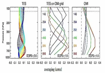
(Zhang, et al., 2010). In fact, this matrix represents vertical resolution of the instrument. In Figure 4 an example of this matrix for each of the two instruments is shown. In this figure, which is related to August 6th in 2006, each line corresponds to a row of averaging kernel. Also, by obtaining the mentioned matrix trace, a number is obtained for each profile that reflects the accuracy of information estimates which is called the degree of freedom of signals (Rodgers, 2000). The profiles extracted from the OMI instrument has a degree of freedom of ozone signals which are DOFS= 6-7 which are in the stratosphere DOFS= 5-7 and in the troposphere is DOFS= 0-1.5. The ozone extraction error in the middle stratosphere is about%1 and about%10 in the troposphere (Liu, et al., 2010). In Figure 4, the signal degree of freedom for the troposphere each OMI and TES profiles are shown. TES averaging kernel shows more sensitivity than OMI which is partly due to the primary precision of the coefficients introduced into the algorithm model of radiation transfer of the instrument (Kulawik, et al., 2006).
Figure 4- An example of the averaging kernel for extracted ozone from TES (left) and OMI (right) at altitudes lower than 100 hPa and in non-cloudy conditions (φ = 28N, λ = 58W). The dash in an
altitude of about 120 hPa represents the boundary layer.
In Figure 4, the middle window shows the re-calculated average core TES on the pressure layers OMI. As it can be seen in the horizontal axis of this window, the new core average values near the surface have substantially improved. Here, the colored numbers are the central pressure of each layer in the OMI algorithm in hPa unit (Zhang, et al., 2010). In continuation, the survey was on the effects of the Solar Zenith Angle to the accuracy of satellite estimates. In Figure 5, the Average Kernel matrices in the 3 Zenith angle (consecutively from left to right) SZA1<30O and 30O<SZA<60O and SZA>60O of the OMI instrument are shown. Here, fc represents the percentage of
cloud presence and αs stands for surface albedo. As seen in the
figure the less is the solar zenith angle the sensitivity to tropospheric ozone increases and the numbers related to average cores in this part of the atmosphere increase. In this figure the dotted line indicates the latitude of the boundary layer (Liu, et al., 2010). The impact of the solar zenith angle on the TES instrument is also likewise in a way that tropospheric ozone
1-Solar Zenith Angle
profiles of the instrument in the form of third-order data processing so that the instrument (4th edition with the networking 2° latitudinal and 4° degrees longitudinal) offered, contained useful information only at latitudes between 50 degrees north-south.
Figure 5 - Effect of changes of the angle of the Solar Zenith on the estimation of the ozone in OMI instrument
4- Validation of Satellite Tropospheric Ozone Column by Ozonesonde
4-1 A comparison between the amount of Satellite Tropospheric Ozone by the Earth equipment and the Increase in the amount of Correlations
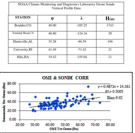
First, 5 sites for sending Ozonesonde balloons were selected based on Table 1and based on the latitude and the kind of area were divided into two groups; the mid-latitude region or tropical and also urban or non-urban. According to this classification, the Hawaii site was set as a site outside of urban areas and free industrial zones, located in the tropical latitudes and four other sites in the urban category, were located in the middle latitudes. It should be noted that all collected data are related to the years 2010 and 2011. On the first step, the total column ozone profiles of OMI instrument from the orbit data of this instrument are extracted from the Ozonesonde coordinates of the urban stations. Then, the latitude of the boundary layer to extract the tropospheric ozone at these profiles was located. Daily data was related to pressure of the boundary layer of the NCEP / NCAR Reanalysis1. According to the World Meteorological Organization definition, the boundary layer is the boundary between the troposphere and the stratosphere, where an abrupt change in lapse rate usually occurs. It is defined as the lowest level at which the lapse rate decreases to 2 °C/km or less, provided that the average lapse rate between this level and all higher levels within 2 km does not exceed 2 °C/km. NCEP data provides the average height of the boundary layer for all days of the year, with 2.5°×2.5° latitude. This data is derived from an average of 4 times measurement per day.
mentioned steps apply for ozone profile data Ozonesonde were also conducted to extract the tropospheric ozone amounts. A comparison of the data that are related to middle-latitude and urban sites is shown in Figure 6.
Table 1 - Features of stations measuring ozone ESRL network
NOAA Climate Monitoring and Diagnostics Laboratory Ozone Sonde Vertical Profile Data
H(m)
λ φ
STATION
1743 -105.25
40.00 Boulder,CO
20 -124.16
40.80 Trinidad Head,CA
196 -86.59
35.28 Huntsville,AL
21 -71.42
41.49 University,RI
11 -155.04
19.43 Hilo,HA
Figure 6- OMI tropospheric ozone and Ozonesonde correlation in urban areas
In this comparison, the correlation coefficient R= 0.548 and the mean variance of tropospheric ozone OMI value obtained by Ozonesonde is 9.02 Dobson. Then the tropospheric ozone amount of TES instrument was obtained also according to the above methods described that the results of validation of these values with Ozonesonde is shown in Figure 7. The results shown in Figures 6 and 7 show the correlation is almost identical to each of the satellite data with data Ozonesonde with this difference that mean variance of tropospheric ozone of TES with Ozonesonde is 4.4 Dobson; approximately half the difference of OMI with Ozonesonde. The next step is to increase the vertical resolution of satellites values of the average of the data and then again compare them with Ozonesonde.
Figure 7- TES tropospheric ozone correlation with Ozonesonde in urban areas
As it is noticed in figure 8, the correlation coefficient R = 0.676 increase this time. As mentioned in section 3 is the increasing correlation of increased vertical resolution.
Figure 8 - tropospheric ozone solidarity OMI/TES and Ozonesonde in urban areas
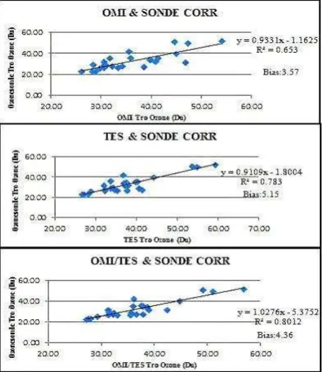
In the next step, all calculations were performed on Hawaii sites, which the results are shown in figure 9. In this area, first, separately, the correlation of each of the instruments with the earth data were analyzed that the correlation coefficient for OMI instrument less than TES instrument and equal to R= 0.808 were calculated, and the coefficient for TES was calculated equal to R= 0.885. Also the mean variance of OMI data with OzoneSode equals 3.57 Dobson this variance for TES instrument was equal to 5:15 Dobson. Then, using satellite data average, the correlation was tested again, and R= 0.895 was obtained, which represents a relative improvement in correlation. By comparing data from each instrument with the
earth’s equipment in rural and urban areas the following results
could be achieved:
• Correlation values for each of the instrument with the earth’s
equipments at tropical latitudes is better middle latitudes because it reduces the vertical resolution of the equator to higher latitudes (increase SZA).
• Correlation values for each of the instrument with the earth’s
equipments in non-urban areas is better than urban areas due to the increase in surface ozone in urban areas and weakness of both instruments in estimating near-surface ozone which causes overestimation of larger amounts in these areas than the reality.
• Combining satellite data increases the solidarity of correlation
with the earth’s equipments, as it causes the increase of the
Figure 9- correlation values of the satellite tropospheric ozone with Ozonesonde in non-urban area
4.2- The Increase or Correlation and the Reduction of the Differences between the Values of Satellite and Terrestrial
As it can be seen in all comparisons conducted, satellite data mean have a positive bias in regard to Ozonesonde data average. The basic hypothesis to reduce this bias is that both
instruments have a low resolution near earth’s surface and actually there isn’t much precision in estimating the amount of
ozone in this section of the atmosphere; however, in non-urban areas that are free of industrial regions and the amount of surface ozone in these areas is minimal, there was a proper correlation between satellite data and Ozonesonde; also, less difference was observed between the mean values of satellite and Ozonesonde and this is true,while in urban areas the correlation is reduced and this difference increased. So it can be concluded that with an increase in surface ozone in the error estimate of both instruments of tropospheric ozone increases. Now, if the effect of existing surface components in urban areas (pre-structure of surface ozone) which cause ozone production could be included in the satellite data and also there would be the possibility of increasing correlations and also reducing the differenced between satellite data and the earth data. To this aim, we will examine the pre-structures of ozone on the surface of the earth, and their mechanism.
Nitrogen oxides in urban areas due to fuel combustion process and consequently cause the exothermic reaction of nitrogen and oxygen in the air. The production of ozone on the surface of the earth is done through the mentioned photochemical reactions of oxides and volatile organic gases in the presence of sunlight and heat.
The equation 2 and 3 show the production of ozone on the surface of the earth:
+ ℎ� + (2)
+ + + (3)
In the equation (3) The component M absorbs the energy from the exothermic reaction and without it, it is impossible to combine molecular and atomic oxygen (Finlayson-Pitts, 2000). To better understand daily changes in ozone on the surface of the earth and its related factors of the clock data of the pollution
monitoring station in Tehran at the position of φ= 35.68 and
=51.34 is used that the results are stated in figure 10.
Figure 10- Hourly Average Annual variations of ozone and nitrogen dioxide in the presence of sunlight (Fath pollution monitoring
station)
This figure represents the average hourly change in ozone,
nitrogen dioxide and (I ↓) downward flux in the time period of
July 2010 to March 2011. In this comparison, the maximum level of ozone is obtained in hour 13 to 15, exactly the time that the amount of nitrogen dioxide reaches its minimum level. Also,
the sun light radiation reaches its maximum level at 12 O’clock
that represents the time required to carry out the photochemical reactions. The continuation of correlation between ozone and nitrogen dioxide is shown in the right window in figure 11 in which the correlation coefficient R= -0.97 is obtained and in the left pane and correlation coefficient of ozone and the downward flux is calculated of R= 0.78.
Figure 11- Ozone correlation with downward flux (left) and nitrogen dioxide (right) (Fath pollution monitoring station)
surface ozone the clock data of the pollution monitoring station
in London with the location features φ= 51.45 and = 0.07 and
the 5 meters sampling height were used. The results of the relationship between the values from January to December in 2010 are shown in Figures 12 and 13. In this survey, also the maximum values of hourly ozone in the range of about 13 to 15 exactly at the range of maximum temperature, with a correlation coefficient R= 0.96 was calculated indicating the important role of temperature in photochemical reactions that produce ozone.
Figure 12- The display of the average hourly annual changes in ozone and temperature (pollution monitoring station
Greenwich-Eltham)
Figure 13- The correlation between ozone and hourly temperature (pollution monitoring station Greenwich-Eltham)
Now, according to all studies conducted to reduce the difference between the amounts of satellite tropospheric ozone with Ozonesonde and also, the increase in their correlation, the math equation shown in Equation 4 was formed:
� � = + + � + �� + (4)
This relationship is written for each satellite common pass and Ozonesonde under the study in each of the sites. In this equation, on the left of the equation is known value of tropospheric ozone derived from Ozonesonde, and on the right was the first term is tropospheric ozone of satellite instruments average in Dobson units, the second term including the amount of tropospheric nitrogen dioxide resulting from OMI instrument in Dobson units, and the third term is downward flux in watts per square meter at the moment of passing satellites, and the fourth term, including the surface temperature derived from the NCEP daily data with networking of 0.25° × 0.25° longitude in degrees kelvin unit and the last term is as a component of the
balanced equation with no unit. In fact, the right side of the 4th equation has two terms originally. One of the satellite tropospheric ozone values and one of the factors contributing to ozone production near the surface to obtain the relative influence of each one of them, all the coefficients of the terms have been calculated. At first, to calculate the unknown factors in the 4th equation, the amounts derived from satellite data and Ozonesode in Hawaii was inserted. These values are related to
26 satellite’s pass, coinciding with Ozonesonde in the time
period of 2010 to 2011 which were written in the in the form of equation 5.The reasons for the selection Hawaii sites for the calculation of the unknown coefficients was the far away distance from the area of industrial pollution and consequently the presence trivial surface ozone and its pre- structures on the
earth’s surface and also latitude of 1λ.43 (near the equator)
which have caused the highest correlation between satellite and the earth data obtained in this area. The 5th equation shows the Ozonesonde matrix values on the left side of the equation and the matrix of information (including tropospheric ozone and nitrogen dioxide satellite values, the surface temperature and downward flux) on the right side with the unknown coefficient matrix. With the help of this connection, the unknown coefficients are calculated. In the next step, the right side of equation 5 for 86 simultaneous passes in four sites of the middle latitudes that all are located in urban areas in the United States, along with the coefficients obtained from the previous step and by multiplying the matrices, a new set of tropospheric ozone values were obtained. The new values are then compared with the values obtained from Ozonesonde and new results were obtained.
[ �+�
⋮ ] = [
� � � � ���
�+ �+ � �+ ���+
⋮ ⋮ ⋮ ⋮ ⋮] ×[ ]
(5)
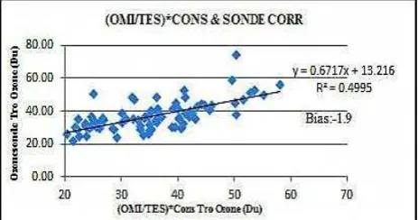
Figure 14 shows the comparison of tropospheric ozone Ozonesonde with satellite values which are multiplied by the values obtained from Hawaii sites. The correlation coefficient R= 0.707 is obtained and it is true if it is in accordance with Figure 7 that the coefficient R= 0.676 for urban areas was obtained. Also the difference between the mean of satellite and Ozonesonde value was calculated at 6.73 Dobson, and this time was reduced to -1.9.
5- Results
In this article, the quality of the tropospheric ozone values derived from satellite instruments and ways to improve them were studied. In the first step, physics both OMI and TES instruments, and also the extraction method of ozone profile in thermal ultraviolet and infrared bands in these instruments were examined. The survey on the averaging kernel matrices of both instruments showed that the accuracy of tropospheric ozone in comparison to stratospheric ozone is much lower. In the next step, to increase the vertical resolution of both instruments in tropospheric ozone of atmosphere, the combined ozone values of both instruments were used and the results were compared with values of ozone obtained from Ozonesode. The results suggest that improving the quality of the satellite data, especially in urban areas. But, nevertheless, still the satellite values have positive bias in comparison with the values
obtained from the earth’s equipments, especially in urban areas
that were studied to reduce the bias effects of the components in the production of surface ozone and these effects in the form of values were multiplied by of satellite tropospheric ozone amounts and new results were obtained. In the final step, again
the results were compared with values obtained from the earth’s
equipment that this comparison revealed a decrease in the bias and correlations were also increased.
Acknowledgement
Thanks to the doctor Haffner in the National Aeronautics and Space Administration's Goddard Space Flight in the US with answer questions, help us to better understand the implications of this knowledge.
References
International Meteorological Vocabulary (2nd ed.)Secretariat of the World Meteorological Organization. (1992). Geneva: p 636-ISBN 92-63-02182-1.
Beer, R. (2006). TES on the Aura Missionμ Scientific
Objectives, Measurements, and Analysis Overview. IEEE TRANSACTIONS ON GEOSCIENCE AND REMOTE SENSING, VOL. 44, NO. 5.
Bowman, K. (et al.,2002). Capturing time and vertical variability of tropospheric ozone: A study using TES nadir retrievals. J.Geophys Res, 107(D23), 4723, doi:10.1029/2002JD002150.
Chance, K. (et al.,1997). Satellite measurements of atmospheric ozone profiles, including tropospheric ozone, from ultraviolet/visible measurements in the nadir geometry:A potential method to retrieve tropospheric ozone. J. Quant. Spectrosc.Radiat. Transfer, 57, 467– 476.
Finlayson-Pitts, B. (2000). Chemistry of the Upper and Lower Atmosphere - Theory, Experiments, and Applications. San Diego, CA.: ISBN: 978-0-12-257060-5.
Jacob, D. (et al.,1999). Introduction to Atmospheric Chemistry. Princeton Univ.
Kulawik, S. (et al.,2006). TES Atmospheric Profile Retrieval
Characterization: An Orbit of Simulated Observations,. IEEE T. Geosci. Remote, P1324-1333. Landgraf, J., & Hasekamp, O. (2007). Retrieval of tropospheric
ozone:The synergistic use of thermal infrared
emission and ultraviolet reflectivity measurements
from space. J.Geophys. Res, VOL. 112, D08310, doi:10.1029/2006JD008097.
Liu, X. (et al.,2010). Ozone profile retrievals from the Ozone
Monitoring Instrument. Atmospheric Chemistry and Physics, P2521-2537.
McPeters, R. (et al.,2007). Ozone climatological profiles for
satellite retrieval algorithms, J. Geophys. Res, 112, D05308.
Nassar, R. (et al.,2008). Validation of Tropospheric Emission Spectrometer (TES) nadir ozones. JOURNAL OF GEOPHYSICAL RESEARCH, VOL. 113.
Park, M. (et al.,2004). Seasonal variations of methane, water vapor, ozone, and nitrogen dioxide near the tropopause: Satellite observations and model simulations. J. Geophys. Res, 109, D03302, doi:10.1029/2003JD003706.
Rodgers, C. (2000). Inverse Methods for Atmospheric Sounding: Theory. World Sci.
Spurr, R. (et al.,2001). Linearized radiative transfer theory: A general discrete ordinate approach to the calculation of radiances and analytic weighting functions, with application to atmospheric remote sensing,Ph.D. thesis,. Technische Universiteit Eindhoven, ISBN 90-386-1789-5.
Worden, J. (et al.,2007). Improved tropospheric ozone profile retrievals using OMI and TES radiances. GEOPHYSICAL RESEARCH LETTERS, VOL. 34, L01809, doi:10.1029/2006GL027806.