Chapter 7 – Input Analysis.pdf

Input Analysis

Input data are key ingredients of simulation modeling. Such data are used to initialize simulation parameters and variables, or construct models of the random components of the system under study. For example, consider a group of milling machines on the shop floor, whose number is to be supplied as a parameter in an input file. You can define a parameter called, say,No_of_Milling_Machinesin the simulation program, and set it to the group size as supplied by the input file. Other examples are target inventory levels, reorder points, and order quantities. On the other hand, arrival streams, service times, times to failure and repair times, and the like are random in nature (see Chapter 3), and are specified via their distributions or probability laws (e.g., Markovian transi-tion probabilities). Such random components must be first modeled as one or more variates, and their values are generated via RNGs as described in Chapter 4.

The activity of modeling random components is called input analysis. From a methodological viewpoint, it is convenient to temporally decompose input analysis into a sequence of stages, each of which involves a particular modeling activity:

Stage 1. Data collection Stage 2. Data analysis

Stage 3. Time series data modeling Stage 4. Goodness-of-fit testing

The reader is reminded, however, that as in any modeling enterprise, this sequence does not necessarily unfold in a strict sequential order; in practice, it may involve multiple backtracking and loops of activities.

Data are the grist to the input analysis mill, and its sources can vary widely. If the system to be modeled already exists, then it can provide the requisite empirical data from field measurements. Otherwise, the analyst must rely on more tenuous data, including intuition, past experience with other systems, expert opinion, or an educated guess. In many real-life applications, expedient heuristics are routinely used. Some of these are mentioned in the following list:

Random variables with negligible variability are simplified and modeled as determi-nistic quantities.

Simulation Modeling and Analysis with Arena

Unknown distributions are postulated to have a particular functional form that incorp-orates any available partial information. For example, if only the distribution range is known (or guessed at), the uniform distribution over that range is often assumed (every value in the range is equally likely). If, in addition, the mode of the distribution is known (or guessed at), then the corresponding triangular distribution is often assumed.

Past experience can sometimes provide information on the functional form of distribu-tions. For example, experience shows that a variety of interarrival times (customers, jobs, demand, and time to machine failure, to name a few) can be assumed to be iid exponentially distributed. The analyst is then only required to fit the rate (or mean) parameter of the exponential distribution to complete the requisite input analysis.

In this chapter we discuss the activities comprising the various stages of input analysis. The ArenaInput Analyzer facilities that support these activities will also be described in some detail. For more information, consult Kelton et al. (2004), Rockwell Software (2005), and the Arena help menus, discussed in Section 6.6.

7.1

DATA COLLECTION

The data collection stage gathers observations of system characteristics over time. While essential to effective modeling, data collection is the first stage to incur modeling risk stemming either from the paucity of available data, or from irrelevant, outdated, or simply erroneous data. It is not difficult to realize that incorrect or insufficient data can easily result in inadequate models, which will almost surely lead to erroneous simula-tion predicsimula-tions. At best, model inadequacy will become painfully clear when the model is validated against empirical performance measures of the system under study; at worst, such inadequacy will go undetected. Consequently, the analyst should exercise caution and patience in collecting adequate data, both qualitatively (data should be correct and relevant) and quantitatively (the sample size collected should be representative and large enough).

To illustrate data collection activities, consider modeling a painting workstation where jobs arrive at random, wait in a buffer until the sprayer is available, and having been sprayed, leave the workstation. Suppose that the spray nozzle can get clogged—

an event that results in a stoppage during which the nozzle is cleaned or replaced. Suppose further that the metric of interest is the expected job delay in the buffer. The data collection activity in this simple case would consist of the following tasks:

1. Collection of job interarrival times. Clock times are recorded on job arrivals and consecutive differences are computed to form the requisite sequence of job interarrival times. If jobs arrive in batches, then the batch sizes per arrival event need to be recorded too. If jobs have sufficiently different arrival characteristics (depending on their type), then the analyst should partition the total arrival stream into substreams of different types, and data collection (of interarrival times and batch sizes) should be carried out separately for each type.

2. Collection of painting times. The processing time is the time it takes to spray a job. Since nozzle cleaning or replacement is modeled separately (see later), the painting time should exclude any downtime.

observations of the effective time to failure should be computed as the time interval between two successive nozzle cloggings minus the total idle time in that interval (if any).

4. Collection of nozzle cleaning/replacement times. This random process is also known as downtime or repair time. Observations should be computed as the time interval from failure (stoppage) onset to the time the cleaning/replacement operation is complete.

It is important to realize that the analyst should only collect data to the extent that they serve project goals. In other words, data should be sufficient for generating the requisite performance statistics, but not more than that. For example, the nozzle-related data collection of items 3 and 4 in the previous list permit the analyst to model uptimes and downtimes separately, and then to generate separate simulation statistics for each. If these statistics, however, were of no interest, then an alternative data collection scheme would be limited to the times spent by jobs in the system from the start of spraying to completion time. These times would of course include nozzle cleaning/ replacement times (if any), but such times could not be deduced from the collected data. The alternative data collection scheme would be easier and cheaper, since less data overall would be collected. Such a reduction in data collection should be employed, so long as the collected data meet the project goals.

Data collection of empirical performance measures (expected delays, utilizations, etc.) in the system under study is essential tomodel validation. Recall that validation checks the credibility of a model, by comparing selected performance measures predicted by the model to their empirical counterparts as measured in the field (see Section 1.5). Such empirical measurements should be routinely collected whenever possible with an eye to future validation. Clearly, validation is not possible if the system being modeled does not already exist. In such cases, the validity of a proposed model remains largely speculative.

7.2

DATA ANALYSIS

Once adequate data are collected, the analyst often performs a preliminary analysis of the data to assist in the next stage of model fitting to data (see Section 7.4). The analysis stage often involves the computation of various empirical statistics from the collected data, including

Statistics related to moments (mean, standard deviation, coefficient of variation, etc.)

Statistics related to distributions (histograms)

Statistics related to temporal dependence (autocorrelations within an empirical time series, or cross-correlations among two or more distinct time series)

These statistics provide the analyst with information on the collected sample, and constitute the empirical statistics against which a proposed model will be evaluated for goodness-of-fit.

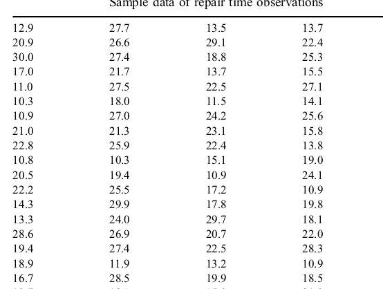
sample, and would usually vary from sample to sample. These statistics (minimum and maximum) play an important role in the choice of a particular (repair time) distribution. Data analysis further discloses that the sample mean is 19.8, the sample standard deviation is 5.76, and the squared sample coefficient of variation is 0.0846. These statistics suggest that repair times have low variability, a fact supported by inspection of Table 7.1.

Arena provides data analysis facilities via its Input Analyzer tool, whose main objective is to fit distributions to a given sample. TheInput Analyzeris accessible from theToolsmenu in the Arena home screen. After opening a new input dialog box (by selecting theNewoption in theFilemenu in theInput Analyzerwindow), raw input data can be selected from two suboptions in theData Fileoption of theFilemenu:

1. Existing data files can be opened via theUse Existingoption.

2. New (synthetic) data files can be created using theGenerate Newoption as iid samples from a user-prescribed distribution. This option is helpful in studying distributions and in comparing alternative distributions.

Once the subsequentInput Analyzerfiles have been created, they can be accessed in the usual way via theOpenoption in theFilemenu.

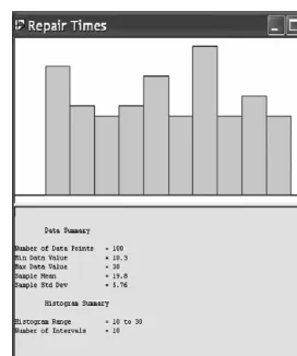
Returning to the repair time data of Table 7.1, and having opened the corresponding data file (calledRepair_Times.dft), theInput Analyzerautomatically creates a histogram from its sample data, and provides a summary of sample statistics, as shown in Figure 7.1.

TheOptionsmenu in theInput Analyzermenu bar allows the analyst to customize a histogram by specifying its number of intervals through theParametersoption and its Histogram option’s dialog box. Once a distribution is fitted to the data (see next section), the same menu also allows the analyst to change the parameter values of the

Table 7.1

Sample data of repair time observations

fitted distribution. TheWindowmenu grants the analyst access to input data (as a list of numbers) via theInput Dataoption.

7.3

MODELING TIME SERIES DATA

The focal point of input analysis is the data modeling stage. In this stage, a proba-bilistic model (stochastic process; see Section 3.9) is fitted to empirical time series data (pairs of time and corresponding observations) collected in Stage 1 (Section 7.1). Examples of empirical observations follow:

An observed sequence of arrival times in a queue. Such arrival processes are often modeled as consisting of iid exponential interarrival times (i.e., a Poisson process; see Section 3.9.2).

An observed sequence of times to failure and the corresponding repair times. The associated uptimes may be modeled as a Poisson process, and the downtimes as a renewal process (see Section 3.9.3) or as a dependent process (e.g., Markovian process; see Section 3.9.4).

Depending on the type of time series data to be modeled, this stage can be broadly classified into two categories:

1. Independent observations are modeled as a sequence of iid random variables (see Section 3.9.1). In this case, the analyst's task is to merely identify (fit) a

“good” distribution and its parameters to the empirical data. Arena provides built-in facilities for fitting distributions to empirical data, and this topic will be discussed later on in Section 7.4.

2. Dependent observationsare modeled as random processes with temporal depend-ence (see Section 3.9). In this case, the analyst's task is to identify (fit) a“good”

probability law to empirical data. This is a far more difficult task than the previous one, and often requires advanced mathematics. Although Arena does not provide facilities for fitting dependent random processes, we will cover this advanced topic in Chapter 10.

We now turn to the subject of fitting a distribution to empirical data, and will focus on two main approaches to this problem:

1. The simplest approach is to construct a histogram from the empirical data (sample), and then normalize it to a step pdf (see Section 3.8.2) or a pmf (see Section 3.7.1), depending on the underlying state space. The obtained pdf or pmf is then declared to be the fitted distribution. The main advantage of this approach is that no assumptions are required on the functional form (shape) of the fitted distribution.

2. The previous approach may reveal (by inspection) that the histogram pdf has a particular functional form (e.g., decreasing, bell shape, etc.). In that case, the analyst may try to obtain a better fit by postulating a particular class of distribu-tions having that shape, and then proceeding to estimate (fit) its parameters from the sample. Two common methods that implement this approach are the method of moments and the maximum likelihood estimation (MLE) method, to be described in the sequel. This approach can be further generalized to multiple functional forms by searching for the best fit among a number of postulated classes of distributions. The Arena Input Analyzer provides facilities for this generalized fitting approach.

We now proceed to describe in some detail the fitting methods of the approach outlined in 2 above, while the Arena facilities that support the generalized approach will be presented in Section 7.4.

7

.

3

.

1

M

ETHOD OF

M

OMENTS

Themethod of momentsfits the moments (see Section 3.5) of a candidate model to sample moments using appropriate empirical statistics as constraints on the candidate model parameters. More specifically, the analyst first decides on the class of distribu-tions to be used in the fitting, and then deduces the requisite parameters from one or more moment equations in which these parameters are the unknowns.

As an example, consider a random variable X and a data sample whose first two moments are estimated asm^1 ¼8:5 andm^2¼125:3. Suppose the analyst decides on

has two parameters (aandb), two equations are needed to determine their values, given ^

m1andm^2above. Using the formulas for the mean and variance of a gamma distribution

in Section 3.8.7, we note the following relations connecting the first two moments of a gamma distribution,m1and m2, and its parameters,aandb, namely,

m1¼ab

m2¼ab2(1þa)

Substituting the estimated values of the two momentsm^1andm^2form1andm2above

yields the system of equations

and this solution completes the specification of the fitted distribution. Note that the same solution can be obtained from an equivalent system of equations, formulated in terms of the gamma distribution mean and variance rather than the gamma moments.

7

.

3

.

2

M

AXIMAL

L

IKELIHOOD

E

STIMATION

M

ETHOD

This method postulates a particular class of distributions (e.g., normal, uniform, exponential, etc.), and then estimates its parameters from the sample, such that the resulting parameters give rise to themaximal likelihood(highest probability or density) of obtaining the sample. More precisely, letf(x;y) be the postulated pdf as function of its ordinary argument,x, as well as the unknown parametery. We mention thatymay actually be a set (vector) of parameters, but for simplicity we assume here that it is scalar. Finally, let (x1,. . .,xN) be a sample of independent observations. The maximal

likelihood estimation (MLE) method estimates y via the likelihood function L(x1,. . .,xN;y), given by

As an example, consider the exponential distribution with parameter y¼l, and derive its maximum likelihood estimate,^y¼^l. The corresponding maximal likelihood function is

ln L(x1,. . .,xN;l)¼N ln l l

XN

i¼1 xi:

The value oflthat maximizes the function lnL(x1,. . .,xN;l) overlis obtained by

differentiating it with respect toland setting the derivative to zero, that is,

d

Solving the above inlyields the maximal likelihood estimate

^

which is simply the sample rate (reciprocal of the sample mean).

As another example, a similar computation for the uniform distribution Unif(a,b) yields the MLE estimates^a¼minfxi: 1iNgand ^b¼maxfxi : 1iNg.

7.4

ARENA

INPUT ANALYZER

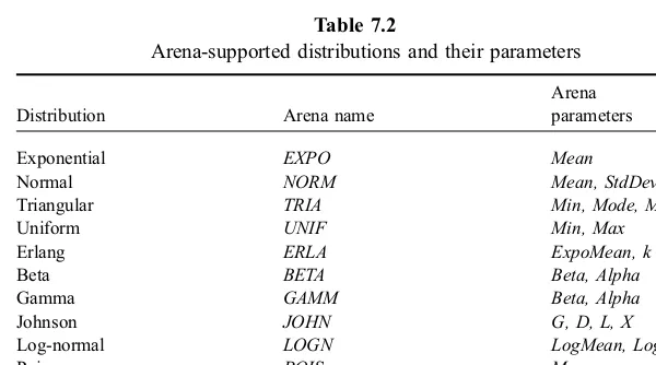
The ArenaInput Analyzerfunctionality includes fitting a distribution to sample data. The user can specify a particular class of distributions and request theInput Analyzer to recommend associated parameters that provide the best fit. Alternatively, the user can request the Input Analyzer to recommend both the class of distributions as well as associated parameters that provide the best fit. Table 7.2 displays the distributions supported by Arena and their associated parameters.

Table 7.2

Note, however, that the parameters in Table 7.2 may differ from those in the corres-ponding distributions of Sections 3.7 and 3.8.

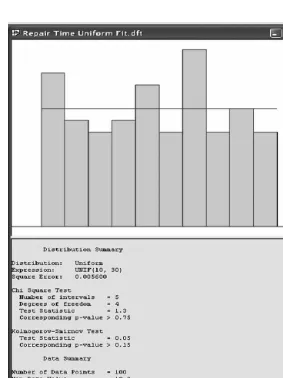
We next illustrate distribution fitting via the Input Analyzer. Suppose the analyst would like to fit a uniform distribution to the data of Table 7.1. To this end, the Repair_Times.dft file (see Section 7.2) is opened from the File menu of the Input Analyzer. TheFitmenu displays all Arena-supported distributions (see Table 7.2), and upon selection of a particular distribution, theInput Analyzercomputes the associated best-fit parameters and displays the results. In our case, Figure 7.2 depicts the output for the best-fit uniform distribution, including the following items:

Graph of the best-fit distribution (pdf ) superimposed on a histogram of the empirical data

Parameters of the best-fit distribution

Statistical outcomes of the goodness-of-fit tests employed (see Section 7.5)

Summary information on the empirical data and the histogram constructed from it.

In our case (best-fit uniform distribution), the associated parameters are just the minimum and maximum of the sample data. TheCurve Fit Summary option of the Windowmenu provides a detailed summary of any selected fit.

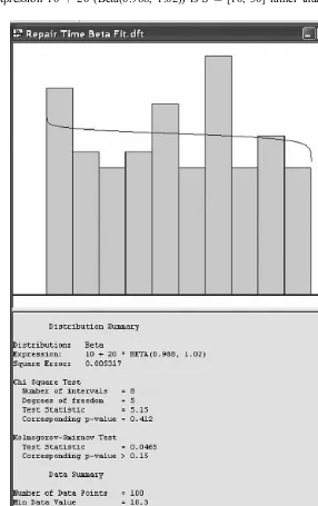
Next, suppose that the analyst changes her mind and would like instead to find the best-fit beta distribution for the same data. Figure 7.3 depicts the resulting Input Analyzeroutput.

Note that the state space of the corresponding random variable, generated via the expression 10þ 20 (Beta(0.988, 1.02)) is S ¼[10, 30] rather than the standard

state space S ¼[0, 1]. Thus, the beta distribution was transformed from the interval [0, 1] to the interval [10, 30] by a linear transformation in the expression above.

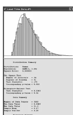
In a similar vein, Figure 7.4 depicts the results of fitting a gamma distribution to a sample of manufacturing lead-time data (not shown). Note theSquare Error field appearing in each summary of the distribution fit. It provides an important measure,e2_,

of the goodness-of-fit of a distribution to an empirical data set, defined by

e2¼X J

j¼1

^ pj pj

2

,

whereJis the number of cells in the empirical histogram,^pjis the relative frequency of

thej-th cell in the empirical histogram, andpj is the fitted distribution's (theoretical)

probability of the corresponding interval. Obviously, the smaller the value ofe2 _{is, the}

better the fit.

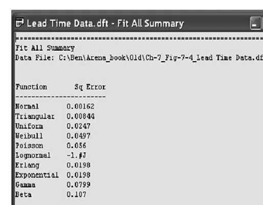
Finally, suppose the analyst would like theInput Analyzerto determine the best-fit distribution overall distribution classessupported by Arena as well as the associated parameters. To this end, theFit Alloption is selected from theFitmenu. In this case, the Fit All Summaryoption may be selected from the Windowmenu to view a list of all classes of fitted distributions and associated square errors, e2, ordered from best to worst (see Figure 7.5).

7.5

GOODNESS-OF-FIT TESTS FOR DISTRIBUTIONS

The goodness-of-fit of a distribution to a sample is assessed by a statistical test (see Section 3.11), where the null hypothesis states that the candidate distribution is a suffi-ciently good fit to the data, while the alternate hypothesis states that it is not. Such statistical procedures serve in an advisory capacity: They need not be used as definitive decision rules, but merely provide guidance and suggestive evidence. In many cases, there is no clear-cut best-fit distribution. Nevertheless, goodness-of-fit tests are useful in providing a quanti-tative measure of goodness-of-fit (see Banks et al. [1999] and Law and Kelton [2000]).

Thechi-square testand theKolmogorov–Smirnov testare the most widely used tests for goodness-of-fit of a distribution to sample data. These tests are used by the Arena Input Analyzerto compute the corresponding test statistic and the associatedp-value (see Section 3.11), and will be reviewed next.

7

.

5

.

1

C

HI

-S

QUARE

T

EST

The chi-square test compares the empirical histogram density constructed from sample data to a candidate theoretical density. Formally, assume that the empirical

sample fx1, . . .,xNg is a set of N iid realizations from an underlying random

variable, X. This sample is then used to construct an empirical histogram with Jcells, where cell j corresponds to the interval½lj,rj). Thus, if Nj is the number of

observations in cellj(for statistical reliability, it is commonly suggested thatNj>5),

then

^ pj¼

Nj

N , j¼1,. . .,J

is the relative frequency of observations in cellj. Letting FX(x) be some theoretical

candidate distribution whose goodness-of-fit is to be assessed, one computes the theoretical probabilities

pj¼PrfljX <rjg, j¼1,. . .,J:

Note that for continuous data, we have

pj¼FX(rj) FX(lj)¼

Note that the quantityNpj is the (theoretical) expected number of observations in cell

jpredicted by the candidate distributionFX(x), whileNjis the actual (empirical) number

of observations in that cell. Consequently, the j-th term on the right side of (7.1) measures a relative deviation of the empirical number of observations in cellj from the theoretical number of observations in cellj. Intuitively, the smaller is the value of the chi-square statistic, the better the fit. Formally, the chi-square statistic is compared against a critical valuec(see Section 3.11), depending on the significance level,a, of the test. Ifw2_{<c, then we accept the null hypothesis (the distribution is an acceptably good fit);}

otherwise, we reject it (the distribution is an unacceptably poor fit). The chi-square critical values are readily available from tables in statistics books. These values are organized by degrees of freedom,d, and significance level,a. The degrees of freedom parameter is given byd ¼J– E – 1, where Eis the distribution-dependent number of parameters estimated from the sample data. For instance, the gamma distribution Gamm(a,b) requires E ¼ 2 parameters to be estimated from the sample, while the exponential distribution Expo(l) only requiresE¼1 parameter. An examination of chi-square tables reveals that for a given number of degrees of freedom, the critical valuecincreases as the significance level,a, decreases. Thus, one can trade off test significance (equivalently, confidence) for test stringency.

Figure 7.1. The best-fit uniform distribution, found by theInput Analyzer, is depicted in Figure 7.2.

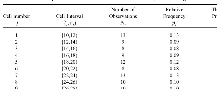
Table 7.3 displays the associated elements of the chi-square test. The table consists of the histogram's cell intervals, number of observations in each cell, and the corresponding empirical relative frequency for each cell. An examination of Table 7.3 reveals that the histogram ranges from a minimal value of 10 to a maximal value of 30, with the individual cell intervals being (10, 12), (12, 14), (14, 16), and so on. Note that the fitted uniform distribution haspj¼0:10 for each cellj. Thus, thew2test statistic is calculated as

w2_¼(13 10) degrees of freedom, the critical value isc¼12.0; recall that the uniform distribution Unif (a,b) has two parameters, estimated from the sample by^a¼minfxi:1iNg ¼10

and^b¼maxfxi:1iNg ¼30, respectively. (When the uniform distribution parameters

aandbare known, thend¼10–1¼9. In fact, the ArenaInput Analyzercomputesdin this manner.) Since the test statistic computed above isw2_{¼3:6<12:0, we accept the null}

hypothesis that the uniform distribution Unif(10, 30) is an acceptably good fit to the sample data of Table 7.1.

It is instructive to follow the best-fit actions taken by the Input Analyzer. First, it calculates the square error

Next, although the histogram was declared to have 10 cells, the Input Analyzer employed a2 _{test statistic with only 6 cells (to increase the number of observations}

in selected cells). It then proceeded to calculate it asw2_{¼2:1, with a correspondingp}

-value ofp > 0.75, clearly indicating that the null hypothesis cannot be rejected even at significance levels as large as 0.75. Thus, we are assured to accept the null hypothesis of a good uniform fit at a comfortably high confidence.

Table 7.3

Empirical and theoretical statistics for the empirical histogram

7

.

5

.

2

K

OLMOGOROV

-S

MIRNOV

(K-S) T

EST

While the chi-square test compares the empirical (observed) histogram pdf or pmf to a candidate (theoretical) counterpart, theKolmogorov-Smirnov (K-S) test compares the empirical cdf to a theoretical counterpart. Consequently, the chi-square test requires a considerable amount of data (to set up a reasonably“smooth”histogram), while the K-S test can get away with smaller samples, since it does not require a histogram.

The K-S test procedure first sorts the sample {x1, x2,. . .,xN} in ascending order

Thus,F^X(x) is just the relative frequency of sample observations not exceeding x. Since

a theoretical fit distributionFX(x) is specified, a reasonable measure of goodness-of-fit

is the largest absolute discrepancy betweenF^X(x) andFX(x). The K-S test statistic is

thus defined by

KS¼max

x fjF^X(x) FX(x)jg: (7:2)

The smaller is the observed value of the K-S statistic, the better the fit.

Critical values for K-S tests depend on the candidate theoretical distribution. Tables of critical values computed for various distributions are scattered in the literature, but are omitted from this book. The ArenaInput Analyzerhas built-in tables of critical values for both the chi-square and K-S tests for all the distributions supported by it (see Table 7.2). Refer to Figures 7.2 through 7.4 for a variety of examples of calculated test statistics.

7.6

MULTIMODAL DISTRIBUTIONS

Recall that the modeof a distribution is that value of its associated pdf or pmf at which the respective function attains a maximal value (a distribution can have more than one mode). Aunimodaldistribution has exactly one mode (distributions can be properly defined to have at least one mode). In contrast, in a multimodal distribution the associated pdf or pmf is of the following form:

It has more than one mode.

It has only one mode, but it is eithernot monotone increasingto the left of its mode, or not monotone decreasingto the right of its mode.

Put more simply, a multimodal distribution has a pdf or pmf with multiple“humps.”

One approach to input analysis of multimodal samples is to separate the sample into mutually exclusive unimodal subsamples and fit a separate distribution to each sub-sample. The fitted models are then combined into a final model according to the relative frequency of each subsample.

As an example, consider a sample of N observations of which N1 observations

appear to form a unimodal distribution in interval I1, andN2 observations appear to

form a unimodal distribution in interval I2, where N1þN2¼N. Suppose that the

theoretical distributionsF1(x) andF2(x) are fitted separately to the respective

FX(x)¼ N1

N F1(x)þ N2

N F2(x): (7:3)

The distributionFX(x) in Eq. 7.3 is a legitimate distribution, which was formed as a

probabilistic mixture of the two distributions,F1(x) andF2(x).

EXERCISES

1. Consider the following downtimes (in minutes) in the painting department of a manufacturing plant.

a. Use the chi-square test to see if the exponential distribution is a good fit to this sample data at the significance levela¼0:05.

b. Using Arena's Input Analyzer, find the best fit to the data. For what range of significance levelsacan the fit be accepted? (Hint: revisit the concept of p-value in Section 3.11.)

2. Consider the following data for the monthly number of stoppages (due to failures or any other reason) in the assembly line of an automotive assembly plant.

Apply the chi-square test to the sample data of stoppages to test the hypothesis that the underlying distribution is Poisson at significance levela¼0:05. 3. Let {xi} be a data set of observations (sample).

a. Show that for the distribution Unif(a,b), the maximal likelihood estimates of the parametersaandbare^a¼minfxigand^b¼maxfxig.

b. What would be the estimates of a and b obtained using the method of moments?

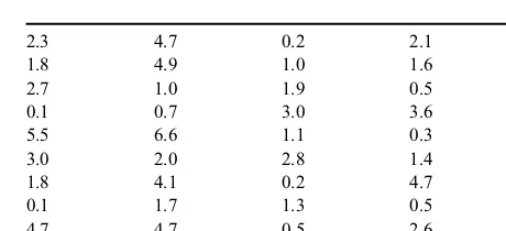
4. The Revised New Brunswick Savings bank has three tellers serving customers in their Highland Park branch. Customers queue up FIFO in a single combined queue for all three tellers. The following data represent observed iid interarrival times (in minutes).

The service times are iid exponentially distributed with a mean of 5 minutes. a. Fit an exponential distribution to the interarrival time data in the previous

table. Then, construct an Arena model for the teller queue at the bank. Run the model for an 8-hour day and estimate the expected customer delay in the teller’s queue.

b. Fit a uniform distribution to the interarrival time data above. Repeat the simulation run with the new interarrival time distribution.

c. Discuss the differences between the results of the scenarios of 4.a and 4.b. What do you think is the reason for the difference between the corresponding mean delay estimates?

d. Rerun the scenario of 4.a with uniformly distributed service times, and com-pare to the results of 4.a and 4.b. Use MLE to obtain the parameters of the service time distribution.

e. Try to deduce general rules from the results of 4.a, 4.b, and 4.d on how variability in the arrival process or the service process affects queue performance measures.

2.3 4.7 0.2 2.1 1.6

1.8 4.9 1.0 1.6 1.0

2.7 1.0 1.9 0.5 0.5

0.1 0.7 3.0 3.6 0.6

5.5 6.6 1.1 0.3 1.4

3.0 2.0 2.8 1.4 2.1

1.8 4.1 0.2 4.7 0.5

0.1 1.7 1.3 0.5 2.2

4.7 4.7 0.5 2.6 2.9