THE EFFECT OF THRESHOLD VALUES ON
ASSOCIATION RULE BASED CLASSIFICATION
ACCURACY
Frans Coenen and Paul Leng
Corresponding Author: Frans Coenen
Department of Computer Science, The University of Liverpool, Liverpool, L69 3BX {frans,phl}@csc.liv.ac.uk
Abstract
Classification Association Rule Mining (CARM) systems operate by applying an
Association Rule Mining (ARM) method to obtain classification rules from a
train-ing set of previously-classified data. The rules thus generated will be influenced by
the choice of ARM parameters employed by the algorithm (typically support and
confidence threshold values). In this paper we examine the effect that this choice
has on the predictive accuracy of CARM methods. We show that the accuracy
can almost always be improved by a suitable choice of parameters, and describe a
hill-climbing method for finding the best parameter settings. We also demonstrate
that the proposed hill-climbing method is most effective when coupled with a fast
CARM algorithm such as the TFPC algorithm which is also described.
Keywords: KDD, Data mining, Classification rule mining, Classification
1
INTRODUCTION
Classification is concerned with the categorisation of records in a data set, typically
achieved by applying a set of Classification Rules (CRs), also sometimes referred to as prediction rules. A classification rule has the general form A → C, where A, the an-tecedent, is the union of some set of attribute values of the records involved: for example
age < 40 and status = married. The consequent, C, is the label of a class to which records can be assigned. Classification rules are typically derived from examination of a
training set of records that have been previously annotated with appropriate class labels.
Many techniques exist to generate CRs from a given training set including techniques based on decision trees [17], Bayesian networks [16], and Support Vector Machines [8].
A method for generating classification rules that has attracted recent attention is
to make use of Association Rule Mining (ARM) techniques. ARM is concerned with the discovery of probabilistic relationships, known as Association Rules (ARs), betweenbinary valued attributes of database records. ARM algorithms, such as Apriori [1], Apriori-TFP
[5] and FPgrowth [12] have been developed specifically to address the problem of finding ARs within very large and sometimes noisy datasets, possibly including very large numbers of attributes.
In general, an AR defines a relationship between disjoint subsets of the overall set of attributes represented by the dataset. For the purpose of obtaining Classification Rules, however, we define binary attributes that represent class-labels, and search only for rules
whose consequent is one of these. To distinguish such specialised ARs from more general ARs we refer to them as Classification Association Rules (CARs).
other CR generation techniques:
• Training of the classifier is generally much faster using CARM techniques than other classification generation techniques such as decision tree and SVM approaches
(particularly when dealing with N classifiers as opposed to binary classifiers).
• Training sets with high dimensionality can be handled very effectively.
• The resulting classifier is expressed as a set of rules which are easily
understand-able and simple to apply to unseen data (an advantage also shared by some other techniques, e.g. decision tree classifiers).
Experimental work has also shown that CARM can offer improved classification accuracy [14]. A significant amount of research effort has therefore been directed at harnessing ARM algorithms to generate CARs. Examples include PRM and CPAR [19], CMAR
[13], CBA [14] and the ARC suite of algorithms [20].
What all of the CARM algorithms that are most frequently referenced in the literature have in common is that they all operate using various parameter thresholds (typically
support and confidence thresholds) and thus their operation is very much dependent on the selection of appropriate values. However, although it is clear that the accuracy of classification will be influenced by the user’s choice of appropriate values for whatever
thresholds are used, most work in applying and evaluating methods of classification makes use of threshold values that are chosen more or less arbitrarily. In this paper we examine the effect of varying the support and confidence thresholds on the accuracy of CARM
to a simplified and more efficient rule-generation process. We describe a hill climbing
algorithm which aims to find the “best” thresholds from examination of the training data. The algorithm is here applied to the support and confidence framework, but can equally well be directed at any other parameters used to generate a classifier. In this
paper we also demonstrate that the proposed hill-climbing method is most effective when coupled with a fast CARM algorithm such as TFPC.
In section 2 we summarise some previous work on CARM, and in section 3 we describe
a new algorithm, TFPC which was introduced briefly in [6] and is here described in detail. In section 4 we describe some experiments that demonstrate the effect of varying the support and confidence thresholds on the accuracy obtained using this and other
algorithms. In section 5 we describe the hill-climbing algorithm, and in section 6 we present results of experiments applying the hill-climbing procedure to TFPC, CBA and CMAR. We show the effect on classification accuracy that can be obtained by a best choice
of thresholds, and discuss how the approach can be applied in practise. Our conclusions are presented in section 7.
2
PREVIOUS WORK
In general, CARM algorithms begin by generating all rules that satisfy at least two user-defined threshold conditions. The support of a rule describes the number of instances in
the training data for which the rule is found to apply. Theconfidenceof the rule is the ratio of its support to the total number of instances of the rule’s antecedent: i.e. it describes the proportion of these instances that were correctly classified by the rule. Minimum threshold
describe too few cases or offer too low classification accuracy. Frequently, however, and
especially when working with imprecise and noisy training data, it will not be possible to obtain a complete classification using only a small number of high-confidence rules. Most methods, therefore, generate a relatively large number of rules which are then pruned.
Algorithms for generating Classification Rules can be broadly categorised according to when the required pruning is performed as follows:
1. Two stage algorithms, which first produce a set of candidate CRs, by a CARM process or otherwise (stage 1). In a separate second stage these are then pruned and ordered for use in the classifier. Examples of this approach include CMAR [13],
CBA [14] and REP as used for example in [15].
2. Integrated algorithmswhere the classifier is produced in a single processing step,
i.e. generation and pruning is “closely coupled”. Examples of this approach include rule induction systems such as FOIL [18], PRM and CPAR [19]. The TFPC algo-rithm, introduced in this paper, also falls into this category. IREP [10] and RIPPER
[7] are one-stage pruning algorithms which may alternatively be applied also as the second stage of a two-stage method.
What all of the above have in common is that they all use various parameter thresholds and thus their operation is very much dependent on the selection of appropriate values. Several of the above methods prune rules bycoverage analysisof the training data. CMAR
[13] uses a threshold for this that determines how many rules are required to cover a case before it is eliminated from the analysis. The FOIL ([18]) algorithm uses thresholds for the number of attributes that can be included in an antecedent and also makes use of a Laplace
minimum gain threshold, a total weight threshold, and a decay factor. Other proposed
measures include Weighted Relative Accuracy (WRA) which in turn reflects a number of rule “interestingness” measures and requires a WRA threshold ([9]). A comparison of interestingness measures used in CARM is presented in Coenen and Leng 2004 ([2]).
Alternatively, some researchers have proposed the use of various heuristics to prune rules (for example [21]).
For further details regarding the above CARM algorithms interested readers are
ad-vised to refer to the indicated references. However, a brief overview of CMAR and CBA is presented in the following two subsections as these are two of the algorithms considered in the experimentation section of this paper.
2.1
CBA (Classification Based on Associations)
The CBA algorithm ([14]) exemplifies the “two-stage” approach, and was one of the first
to make use of a general ARM algorithm for the first stage. CBA uses a version of the well-known Apriori algorithm [1], using user supplied support and confidence thresholds, to generate CARS which are then prioritised as follows (given two rules r1 and r2):
1. r1 has priority over r2 ifr1.conf idence > r2.conf idence.
2. r1 has priority over r2 if r1.conf idence == r2.conf idence and r1.support > r2.support.
3. r1 has priority over r2 if r1.conf idence == r2.conf idence and r1.support ==
r2.support and |r1.antecedent|<|r2.antecedent|.
1. For each record d in the training set find the first rule (the one with the highest
precedence) that correctly classifies the record (the cRule) and the first rule that wrongly classifies the record (the wRule).
2. For each record where the cRulehas higher precedence than the wRule, the rule is included in the classifier.
3. For all records where the cRule does not have higher precedence than the wRule
alternative rules with lower precedence must be considered and added to the classi-fier.
CRs are added to the classifier according to their precedence. On completion the lower precedence rules are examined and a default rule selected to replace these low precedence CRs. CBA illustrates a general performance drawback of two-stage algorithms; the cost of
the pruning stage is a product of the size of the data set and the number of candidate rules, both of which may in some cases be large. It is clear, also, that the choice of support and confidence thresholds will strongly influence the operation of CBA. The ordering strategy
seems to work well on some data sets but less well on others.
2.2
CMAR (Classification based on Multiple Association Rules)
The CMAR algorithm ([13]) has a similar general structure to CBA, and uses the same CR prioritisation approach as that employed in CBA. CMAR differs in the method used
in stage 1 to generate candidate rules, which makes use of the FP-tree data structure coupled with the FP-growth algorithm [12]; this makes it more computationally efficient than CBA. Like CBA, CMAR tends to generate a large number of candidate rules. The
and all rules where a more general rule with higher precedence exists. Finally, a database
coverage procedure is used to produce the final set of rules. This stage is similar to that of CBA, but whereas CBA finds only one rule to cover each case, CMAR uses a coverage threshold parameter to generate a larger number of rules. When classifying an
“unseen” data record, CMAR groups rules that satisfy the record according to their class and determines the combined effect of the rules in each group using a Weighted χSquared (WCS) measure.
3
TOTAL FROM PARTIAL CLASSIFICATION
The methods referenced above perform some form of coverage analysis, either as a separate
phase or integrated into the rule-generation process, to verify the applicability of rules generated to the cases in the training data. The cost of this analysis, especially when dealing with large data sets with many attributes and multiple cases, motivated us to consider whether it is possible to generate an acceptably accurate set of Classification
Rules directly from an ARM process, without further coverage analysis. The TFPC algorithm 1 described here is directed at this aim. The principal advantage offered by TFPC, with respect to threshold tuning using the hill climbing approach described later
in this paper, is that it is extremely efficient (because it dispenses with the need for coverage analysis).
TFPC is derived from a general ARM algorithm, Apriori-TFP, that we have described elsewhere [5]. We assume that database records (transactions) comprise the values of a set of binary attributes; data not in this form is first discretised to make it so. A transaction
1TFPC may be obtained fromhttp://www.csc.liv.ac.uk/
may then be said to “contain” the items corresponding to the non-zero attribute values
present. Apriori-TFP finds in this data all the “frequent” sets, ie sets of items whose occurrence in the data reaches a defined threshold of support. The method makes use of two set-enumeration tree structures for this purpose. In a single pass of the data, the
data is first transcribed into a structure we call the P-tree, first described in [11], which contains a Partialsummation of relevant support-counts. The P-tree orders sets of items according to some defined ordering of the single items, so that each subtree contains only
following supersets of its root node. Previous work has shown that the algorithm works most efficiently if items are placed in descending order of their frequency in the data set [3]. As each record in the data is examined, the set of items it contains is inserted into
the P-tree. If a node representing the set already exists, its support count is incremented; otherwise a new node is created. When two nodes added to the tree share a common prefix, this prefix is used to create a new parent node for them if this does not already
exist. These additional nodes are required to prevent the tree degenerating into a list structure. The final P-tree, however, is of the same order of size as the original database, and may be smaller if there are duplicate records.
As each database record (a set of items) is considered, the current tree is traversed to find the position of the node at which this itemset is placed and counted. During this traversal, the algorithm examines each preceding subset of the node that is found in
the tree, and adds to the count of this. The effect is that in the final P-tree, the count recorded at each node is a summation of the counts of all nodes in the subtree of which it is the root, i.e. of all the supersets that follow it in the set ordering.
in time and conservative in space requirements. To complete the generation of frequent
sets, we apply a second stage of the algorithm that builds a second set-enumeration tree structure which we call the T-tree (Total support tree). Like the P-tree, the T-tree stores itemsets at nodes such that each subtree contains only supersets of its parent node, but
in this case the nodes in the subtree are those that precede their parent according to the ordering of itemsets. The T-tree is constructed by a breadth-first iterative process that ends with a tree that contains only the frequent sets.
The TFPC algorithm adapts these structures and procedures to the task of generating classification association rules. For this purpose, class labels are defined as items, and placed at the end of the ordering of items. The first stage of the algorithm then constructs
a P-tree that contains partial counts of all the sets of items that have been found in records labelled with one or other of these classes.
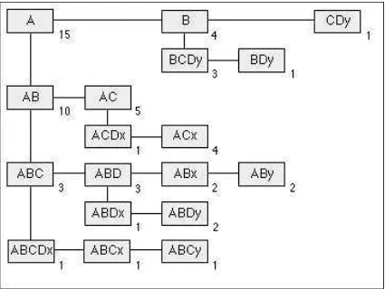
To illustrate this, consider a dataset of records each of which comprises some subset
of the attribute-set A, B, C, D that is labelled with a class-label, x or y. For clarity and simplicity, we will use the notation ACDx, for example, to represent a record with attributes A,C and D, which has been placed in class x. The training set comprises the
following instances: ABCDx, ABCx, ABCy, ABDx, ABDy, ABDy, ABx, ABy, ABx, ABy, ACDx, ACx, ACx, ACx, ACx, BCDy, BCDy, BCDy, BDy, CDy. Figure 1 illustrates the P-tree that would be constructed from this data. Rather than the conventional tree
rep-resentation, we represent child nodes of each parent as an ordered linked list, illustrating the actual form of the implementation. The form of the final tree is independent of the order in which the data is presented. Notice that the leaf nodes of the tree each represent
yet a full support-count; for example, the count recorded for AC (5) does not incorporate
the count for the sets in the subtree rooted at ABC.
To complete the counting of support, a minimum support threshold is chosen and a T-tree is constructed. Figure 2 illustrates the tree that would result from this data, with
a support threshold of 30%. The T-tree is built level by level, starting with nodes that represent single items. In this case, the first level comprises the items A, B, C, and D, and the class-labels x and y. The P-tree is traversed once to obtain complete
support-counts for all of these: for example the overall support-count for B (14) is the sum of the partial counts for the sets B (4) and AB (10) found in the P-tree. After completing the first level, a second level comprising pairs of items is added to the tree. Here, each
pair is appended to the parent representing its second item, so the subtrees now contain preceding supersets of their root. The support of these sets is counted, and the process repeated for the third and subsequent levels. At each stage, sets are added to the tree
only if all their subsets reach the required threshold of support, and are pruned if they are found to lack the necessary support. For example, in this case the set AD will initially have been appended to the tree. The total number of instances of AD in the data, (5),
does not reach the support threshold (30%, or 6 cases), so this node is pruned after level 2 is counted, and the supersets of AD are not added to the tree at level 3. This procedure, of course, replicates the well-known Apriori methodology, albeit using a more efficient
counting algorithm that makes use of the tree structures and the counting already done in constructing the P-tree. The process continues until no more nodes can be added. The final T-tree contains all the frequent sets with their support-counts.
classifica-tion rules, an addiclassifica-tional form of pruning is applied, using the chosen confidence threshold.
Each set appended to the subtrees rooted at x and y defines a possible Classification Rule: for example, the node labelledCxleads to a ruleC→x, with confidence 7/12 (ie support of Cx/support of C). Whenever a candidate rule of this kind is found to reach the
re-quired support threshold, TFPC calculates its confidence, and if this reaches the rere-quired confidence threshold, the set is removed from the tree and added to the target set of CRs. The effect of this is that no further supersets of the set from which the rule is derived are
added to the tree. For example, suppose we define a confidence threshold of 70% for the data illustrated. The set Dy leads to a rule D → y, with confidence 7/10, which meets this threshold, so the rule would be accepted. In this event the set Dy would be removed
from the tree and the set BDy would not be appended.
This pruning heuristic has two desirable consequences. The first is that fewer sets need to be counted, significantly improving the speed of the rule-generation algorithm. The
second is that fewer final rules will be generated, as once a general rule of sufficient confi-dence is found, no more specific rules (rules with the same consequent, whose antecedent is a superset) will be considered. This “on-the-fly” pruning replaces the expensive pruning
step that other algorithms perform by coverage analysis.
Table 1 summarises the rule-generation algorithm. When applying the rules to classify unseen data, the rule set is sorted first by confidence, then by support. Between two rules
of equal confidence and support, the more specific takes precedence. This differs from the precedence used in CBA and other algorithms, which favours more general rules on the basis that prioritising more specific rules may lead to overfitting. In our case, however,
specific rules compensates for the initial preference given to general rules. Optionally,
also, we may terminate the T-tree construction at a defined depth, to limit the maximum size of rule-antecedents.
TFPC provides a very efficient algorithm for generating a relatively compact set of
CRs. Because no coverage analysis is carried out, however, the choice of appropriate support and confidence thresholds is critical in determining the size of the final rule set. In the next section we examine the effect of varying these thresholds on this and other
algorithms.
4
The effect of varying threshold values
To examine the effect that may result from different choices of threshold values, we carried out a series of experiments using test data from the UCI Machine Learning Repository. The data sets chosen were discretized using the LUCS-KDD DN software 2. In the dis-cussion and illustrations that follow, we identify each data set with a label that describes
its key characteristics, in the form in which we have discretized it. For example, the label glass.D48.N214.C7 refers to the “glass” data set, which includes 214 records in 7 classes, with attributes which for our experiments have been discretised into 48 binary
categories.
Using this data, we investigated the classification accuracy that can be achieved using
the TFPC algorithm, and also from CMAR and CBA, across the full range of values for the support and confidence thresholds. For each pair (support, confidence) of threshold
2Available athttp ://www.csc.liv.ac.uk/
∼f rans/KDD/Sof tware/LU CS−KDD−DN/lucs−
values we obtained a classification accuracy from a division of the full data set into a
90% training set and 10% test set. All the implementations were written in Java 1.4 by the authors. Experiments were conducted using a single Celeron 1.2 GHz CPU with 512 MBytes of RAM. The results for a selection of the data sets considered are illustrated in
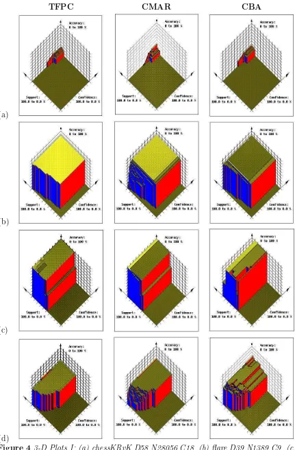
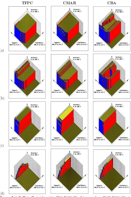
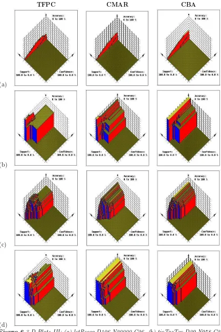
Figures 4, 5 and 6 (presented at the end of this paper) in the form of 3-D plots. For each plot the X and Y axes represent support and confidence threshold values from 100% to 0%, and the Z axis the corresponding percentage classification accuracy obtained.
In these figures,the first illustration in each row is the plot for the TFPC algorithm. These results demonstrate a range of different characteristics of the various data sets. In some cases, for example flare, the best accuracy is obtained for a very broad range
of threshold values. These represent “easy” cases to classify: those in which all the necessary rules have high support and confidence in the training data. In other cases, conversely, such as led7, and letRecog the accuracy obtained is very sensitive to the
choice of thresholds. Even in cases where a near-best accuracy is easily obtained, there may be small regions in the search space where a better result can be achieved: hepatitis and heart are examples. Generally, the best accuracy is obtained using a low support
threshold, but there are cases where this is not so. Usually, these arise when the training set is small so that rules with low support may represent very few cases: see, for example
iris and wine. The choice of confidence threshold, however, is often more critical. Our experiments include cases (e.g. ticTacToe and waveform) where a high confidence threshold is required. These represent cases where TFPC can perform badly if a low confidence threshold is chosen, because a rule that meets this threshold may mean that
and chess are examples. Usually these are data sets for which classification accuracy is
low, and only low-confidence rules can be found.
The plots for CMAR (second illustration in each row) have a broadly similar pattern. The illustrations show, however, the way in which the coverage analysis smooths out some
of the influence of the choice of threshold. led7, iris and wine, all cases that for TFPC are sensitive to the thresholds of support and/or confidence, are good examples of this. In these cases, provided sufficiently low thresholds are chosen, then CMAR will find all the
necessary candidate rules, and the coverage analysis reliably selects the best ones. This smoothing effect is not perfect, however; note that foriris, CMAR still has a suboptimal result if a very low support threshold is chosen, and the examples of ticTacToe and
ionosphereillustrate cases where a choice of a low confidence threshold will lead to poor rules being selected. Conversely, in cases such as letRecog and chess, where few if any high-confidence rules can be found, a low confidence threshold is again needed to find
candidate rules.
The illustrations for CBA also, in many cases, demonstrate the “smoothing” effect obtained as a result of applying coverage analysis to select rules from the initial candidates.
This is especially to be seen in some of the larger data sets: letRecog, ticTacToe and
waveformall illustrate cases where CBA’s accuracy is more stable than that of CMAR. In other cases, however, usually involving small data sets, CBA may be even more sensitive
than TFPC to the choice of thresholds. The examples of hepatitis and ionosphere are especially interesting: in both cases, a poor choice of thresholds (even values that appear reasonable) may lead to a dramatically worse result. This is partly because, unlike CMAR,
enough for these to reach the required thresholds.
5
Finding best threshold values
It is clear from the experiments discussed above that the accuracy and performance of both TFPC, in particular, and rule-generation algorithms in general, may be very sensitive
to the choice of threshold values used. The coverage analysis used by methods such as CMAR and CBA sometimes reduces this sensitivity, but does not eliminate it. It is apparent that the accuracy of the classifiers obtained using any of these methods may be
improved by a careful selection of these thresholds.
In this section we describe a procedure for identifying the “best” threshold values, i.e,
those that lead to the highest classification accuracy, from a particular training set. The method applies a “hill-climbing” strategy, seeking to maximise accuracy while varying the thresholds concerned. We will describe this in relation to thresholds of support and confidence, although the method can be applied in general to other kinds of threshold
also.
The hill climbing technique makes use of a 3-D playing area measuring 100×100× 100, as visualised in Figures 4, 5 and 6. The axes of the playing area represent: (1)
support thresholds, (2) confidence thresholds and (3) accuracies (all defined in terms of percentages). The procedure commences with initial support and confidence threshold
values, describing a current location (cl) in the base plane of the playing area. Using these values, the chosen rule-generation algorithm is applied to the training data, and the resulting classifier applied to the test data, with appropriate cross-validation, to obtain a
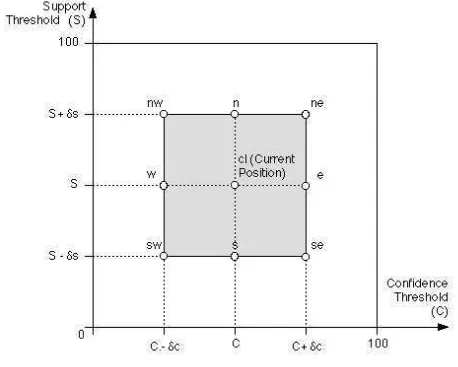
The hill-climbing procedure then attempts to move round the playing area with the
aim of improving the accuracy value. To do this it continuously generates data for a set of eight test locations — hence the term 8 point hill climbing. The test locations are defined by applying two values, δS (change in support threshold) and δC (change in confidence
threshold), as positive and negative increments of the support and confidence threshold values associated with cl. The current and test locations form a two dimensional 3×3 location grid with cl at the center (Figure 3). The test locations are labelled: n, ne, e,
se, s, sw, w, nw and n, with the obvious interpretations. The objective here is to avoid finding local minima as featured in some of the plots identified in Figures 4, 5 and 6.
The rule-generation algorithm is applied to each of the test locations which is inside
the playing area and for which no accuracy value has previously been calculated. A classification accuracy is thus obtained for each location. If this stage identifies a point with a superior accuracy to the current cl, the procedure continues withcl as this point.
Between candidate points of equal accuracy, the algorithm uses a weighting procedure to select a “best” point from which to continue. If the current cl has the best accuracy, then the threshold increments are reduced and a further iteration of test locations takes
place. The process concludes when either: (i) a best accuracy is obtained or (ii) a lower limit on the threshold-increments is reached at which point the current pair of threshold values which leads to a “best” classification accuracy for the chosen training and test data
are selected. This will not always be a true best value, depending on the choice of the initial cl and other parameters, but will at worst be a local optimum. The hill climbing procedure is summarised in Table 2. It should be noted that the hill climbing is performed
6
RESULTS
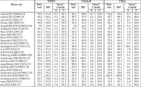
Table 3 summarises the results of applying the hill-climbing procedure described above
to datasets from the UCI repository, for the algorithms TFPC, CMAR and CBA. For each algorithm, the first two columns in the table show the average accuracy obtained from applying the algorithm to (90%, 10%) divisions of the dataset with ten-fold
cross-validation. The first of the two columns shows the result for a support threshold of 1% and a confidence threshold of 50% (the values usually chosen in analysis of classification algorithms), and the second after applying the hill-climbing procedure to identify the
“best” threshold values. Note that, with respect to the experiments. δS andδC were set to 6.4 and 8.0 respectively, and minδS and minδC to 0.1 and 1.0; as these parameters were found to give the most effective operational results. The support and confidence
threshold values selected to obtain the best accuracy are also tabulated.
Table 3 confirms the picture suggested by the illustrations in Figures 4, 5 and 6 (although note the correspondence is not always exact, as cross-validation was not used in
obtaining the graphical representations — see Section 4). In almost all cases, an improved accuracy can be obtained from a pair of thresholds different from the default (1%, 50%) choice. As would be expected, the greatest gain from the hill-climbing procedure is in
the case of TFPC, but a better accuracy is also obtained for CMAR in 21 of the 25 sets, and for CBA in 20. In a number of cases the improvement is substantial. It is apparent that CBA, especially, can give very poor results with the default threshold values. In the
includes misleading instances if a small support threshold is chosen. In the latter case the
hill-climbing procedure has been ineffective in climbing out of the deep trough shown in the illustration for CBA. Notice that here the coverage analysis used in CMAR is much more successful in identifying the best rules, although TFPC also does relatively well.
As we observed from the illustrations, and as results reported in [13] also show, CMAR is generally less sensitive to the choice of thresholds. Both CMAR and CBA, however, give very poor results when, as in the cases of chessandletrecog, the chosen confidence
threshold is too high, and CMAR performs relatively poorly forled7for the same reason. The extreme case is chess, where both CMAR and CBA (and TFPC) find no rules at the 50% confidence threshold. Notice, also, that for the largest data sets (those with
more than 5000 cases) a support threshold lower than 1% almost always produces better results, although the additional candidate rules generated at this level will make coverage analysis more expensive.
In general, the results show that coverage analysis, especially in CMAR, is usually (although not always) effective in minimising any adverse effect from a poor choice of thresholds. Although TFPC with the default threshold values produces reasonably high
accuracy in most cases, the lack of coverage analysis generally leads to somewhat lower accuracy than one or both of the other methods. Interestingly, however, the results when the hill-climbing procedure is applied to TFPC show that high accuracy can be obtained
without coverage analysis if a good choice of thresholds is made. In 18 of the 25 cases, the accuracy of TFPC after hill-climbing is as good or better than that of CMAR with the default thresholds, and in only one case (wine) is it substantially worse, the
hill-climbing procedure of TFPC works better than the coverage analysis of CMAR in
identifying important low-support, high-confidence rules. The results also improve on CBA in 14 cases, often by a large margin. Overall this suggests that a good choice of thresholds can eliminate the need for coverage analysis procedures.
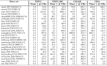
The significance of this is that coverage analysis is relatively expensive, especially if the data set and/or the number of candidate rules is large, as is likely to be the case if a low support threshold is chosen. Table 4 gives a comparison of the total execution
times to construct a classifier with ten-fold cross validation, using TFPC, with or without the hill-climbing procedure, and for CMAR and CBA (for the 1%, 50% thresholds). The average number of rules generated in each case is also shown. These figures were obtained
using the author’s Java implementations of the algorithms running on single Celeron 1.2 Ghz CPU with 512 MBytes of RAM.
As would be expected, the execution times for TFPC (with default threshold values)
are almost always far lower than for either of the other two methods. Less obviously, performing hill-climbing with TFPC is in many cases faster than coverage analysis with CMAR or CBA. In 13 of the 25 cases, this was the fastest procedure to obtain classification
rules, and it is only markedly worse in cases such aschessandletRecog, where the other methods have failed to identify the rules necessary for good classification accuracy.
TFPC also, in most cases, generates fewer rules that CMAR, leading to faster
oper-ation of the resulting classifier. The case of flare is interesting in this respect. Here, a single rule is sufficient to identify 84.3% of cases; both CMAR and CBA find select many more rules, but without improving on this accuracy. Together with the results shown in
7
CONCLUSIONS
In this paper we have shown that the choice of appropriate values for the support and
confidence thresholds can have a significant effect on the accuracy of classifiers obtained by CARM algorithms. The coverage analysis performed by methods such as CMAR and CBA reduces this effect, but does not eliminate it. CMAR appears to be less sensitive
than CBA to the choice of threshold values, but for both methods better accuracy can almost always be obtained by a good choice. We have also shown that, if threshold values are selected well, it is possible to obtain good classification rules using a simple and fast
algorithm, TFPC, without the need for coverage analysis. We describe a procedure for finding these threshold values that will lead to good classification accuracy. Our results demonstrate that this approach can lead to improved classification accuracy, at a cost
that is comparable to or lower than that of coverage analysis. The technique can be applied to all the currently popular CARM algorithms as illustrated in the paper using the well known CMAR and CBA algorithms — the authors would therefore suggest that
the results obtained are generalisable. It should also be noted that the hill climbing technique is not dependent on specific properties of the P and T trees used in the TFPC algorithm, although use of TFPC does make the approach more computationally effective.
References
[1] R. Agrawal and R. Srikant, Fast algorithms for mining association rules, in Proc. 20th
VLDB Conference (Morgan Kaufman, 1994) 487-499.
[2] F. Coenen and P. Leng, An evaluation of approaches for classification rule selection,
[3] F. Coenen and P. Leng, Optimising Association Rule Algorithms using itemset
order-ing, In Proc ES2002 conference (Springer, 2002) 53-66.
[4] F. Coenen and P. Leng, Data Structures for Association Rule Mining T-trees and
P-trees, IEEE Transactions on Knowledge and Data Engineering 16(6)(2004) 774-778.
[5] F. Coenen, P. Leng and G. Goulbourne, Tree Structures for Mining Association Rules, Journal of Data Mining and Knowledge Discovery, Vol 8 (1)(2004) 25-51.
[6] F. Coenen, P. Leng and L. Zhang, Threshold Tuning for Improved Classification As-sociation Rule Mining, in Proc. PAKDD 2005 conference (Springer LNAI3158, 2005), 216-225.
[7] W.W. Cohen, Fast Effective Rule Induction, in Proc. 12th Int. Conf. on Machine Learning (Morgan Kaufmann, 1995), 115-123.
[8] N. Christianin and J. Shawe-Taylor, An Introduction to Support Vector Machines and
Other Kernel-Based Learning Methods, (Cambridge University Press, 2000).
[9] N. Lavraˇc, P. Flach and B. Zupan, Rule Evaluation Measures: A Unifying View, in Proc. Ninth International Workshop on Inductive Logic Programming (ILP’99) (Springer-Verlag 1999), 174-185.
[10] J. F¨urnkranz, J. and F. Widme, Incremental reduced error pruning, in Proc. 11th Int. Conf. on Machine Learning (Morgan Kaufmann, 1994), pp70-77.
[11] G. Goulbourne, F. Coenen and P. Leng, Algorithms for Computing Association Rules using a Partial Support Tree, in Proc ES99 Conference (Springer 1999), 132-147; also
[12] J. Han., J. Pei, and Y. Yin, Mining Frequent Patterns without Candidate generation,
Proc ACM Sigmod conf, (2000) 1-12.
[13] W. Li, J. Han and J. Pei, CMAR: Accurate and Efficient Classification Based on
Multiple Class-Association Rules, in Proc. ICDM 2001 conference (IEEE 2001), 369-376.
[14] B. Liu, W. Hsu and Y. Ma, Integrating Classification and Association Rule Mining, in Proc. KDD-98 conference (AAAI 1998), 80-86.
[15] G. Pagallo and D. Haussler, Boolean feature discovery in Empirical data, Machine Learning, 5(1) (1990), 71-99.
[16] J. Pearl, Probabilistic Reasoning in Intelligent Systems, (Morgan Kaufmann, San Mateo 1998).
[17] J.R. Quinlan, Induction of decision trees, Machine Learning (1) (1986), 81-106.
[18] J.R. Quinlan and R.M. Cameron-Jones, FOIL: A Midterm Report. on Proc. ECML
conference (1993), 3-20.
[19] X. Yin and J. Han, CPAR: Classification based on Predictive Association Rules, in
Proc. SIAM Int. Conf. on Data Mining (SDM’03) (2003) 331-335.
[20] O.R. Zaiane and M-L. Antonie, Text Document Categorization by Term Association,
on Proc. ICDM’2002 conference (IEEE 2002),19-26.
Inputs: Data set D, support thresholds, confidence thresholdc
Output: Set of CRs R
Preprocess input data so that:
i) Unsupported attributes are removed, and
ii) Recast records so that remaining attributes (not classes) are ordered according to frequency.
Create a P-tree
Create level 1 of T-tree (single items)and count supports by traversing P-tree Generate level 2 of T-trees (the 2-item candidate sets)
R ←null K ←2 Loop
pass through P-tree to obtain support counts for level K
remove unsupported elements in level K
for all remaining elements in level K in branches representing a class, generate a CR with associated confidence value: if (conf idence > c)
R←R∪CR
remove corresponding level K element from tree End if
K ←K+ 1
Generate level K nodes (the K candidate itemsets) from the remaining K−1 itemsets using the downward closure property of itemsets
if no level K nodes generated break
End loop
Algorithm: 8-Point Hill Climbing input A Training and Test data setD, and
a Rule Generation Algorithm RGA
ApplyRGA toD using thresholds cl.S and cl.C
Evaluate ruleset generated to determine accuracy cl.accuracy Start loop
Apply δS, δC tocl.S, cl.C to generate test pointsP
Apply RGA to determine accuracy for all points not previously evaluated
bl←location with best accuracy in P
If bl is unique then
Ifbl=cl Then δS ←δS/2,δC ←δC/2 Else cl←bl
Else If majority of P have best accuracy Then
TFPC CMAR CBA
Data set Def. “best” Def. “best” Def. “best”
val. HC t’hold val. HC t’hold val. HC t’hold
S C S C S C
adult.D97.N48842.C2 80.8 81.0 0.2 50.1 80.1 80.9 0.7 50.0 84.2 84.6 0.1 48.4 anneal.D73.N898.C6 88.3 90.1 0.4 49.1 90.7 91.8 0.4 50.0 94.7 96.5 0.8 46.8 auto.D137.N205.C7 70.6 75.1 2.0 52.4 79.5 80.0 1.2 50.0 45.5 77.5 2.7 50.8 breast.D20.N699.C2 90.0 90.0 1.0 50.0 91.2 91.2 1.0 50.0 94.1 94.1 1.0 50.0 chessKRK.D58.N28056.C18 0.0 38.0 0.1 25.2 0.0 34.6 0.1 11.0 0.0 39.8 0.1 24.0 cylBands.D124.N540.C2 68.3 74.4 1.2 49.8 75.7 77.8 1.3 49.9 75.7 78.0 1.9 50.0 flare.D39.N1389.C9 84.3 84.3 1.0 50.0 84.3 84.3 1.0 50.0 84.2 84.2 1.0 50.0 glass.D48.N214.C7 64.5 76.2 2.6 45.6 75.0 75.0 1.0 50.0 68.3 70.7 3.0 51.6 heart.D52.N303.C5 51.4 56.0 4.2 52.4 54.4 54.8 1.6 50.0 57.3 60.0 4.2 49.2 hepatitis.D56.N155.C2 81.2 83.8 1.6 51.6 81.0 82.8 2.9 50.0 57.8 83.8 7.1 48.4 horseColic.D85.D368.C2 79.1 79.9 1.2 50.2 81.1 81.9 2.9 50.0 79.2 83.9 5.5 49.2 ionosphere.D157.N351.C2 85.2 92.9 9.8 50.0 90.6 91.5 2.6 50.0 31.6 89.5 10.0 49.2 iris.D19.N150.C3 95.3 95.3 1.0 50.0 93.3 94.7 2.3 50.0 94.0 94.0 1.0 50.0 led7.D24.N3200.C10 57.3 62.7 2.2 49.4 62.2 67.4 1.3 40.4 66.6 68.0 1.0 46.0 letRecog.D106.N20000.C26 26.4 47.6 0.1 32.3 25.5 45.5 0.1 31.8 28.6 58.9 0.1 13.7 mushroom.D90.N8124.C2 99.0 99.7 1.8 69.2 100.0 100.0 1.0 50.0 46.7 46.7 1.0 50.0 nursery.D32.N12960.C5 77.8 89.9 1.0 73.2 88.3 90.1 0.8 62.6 90.1 91.2 1.5 50.0 pageBlocks.D46.N5473.C5 90.0 90.0 1.0 50.0 90.0 90.3 0.2 50.0 90.9 91.0 1.6 50.0 penDig.D89.N10992.C10 81.7 88.5 0.1 62.3 83.5 85.2 0.8 50.0 87.4 91.4 0.1 50.9 pima.D38.N768.C2 74.4 74.9 2.3 50.0 74.4 74.5 1.6 50.0 75.0 75.7 2.8 50.0 soybeanLrg.D118.N683.C19 89.1 91.4 1.1 49.1 90.8 91.8 0.8 51.6 91.0 92.9 0.6 52.2 ticTacToe.D29.N958.C2 67.1 96.5 1.5 74.2 93.5 94.4 1.6 50.0 100.0 100.0 1.0 50.0 waveform.D101.N5000.C3 66.7 76.6 3.2 64.3 76.2 77.2 0.6 50.0 77.6 78.2 2.6 50.0 wine.D68.N178.C3 72.1 81.9 4.5 51.2 93.1 94.3 2.3 50.0 53.2 65.5 4.8 50.0 zoo.D42.N101.C7 93.0 94.0 1.0 49.2 94.0 95.0 1.6 50.0 40.4 93.1 7.4 50.0
Data set TFPC TFPC-HC CMAR CBA
Time # CRs Time # CRs Time # CRs Time # CRs
adult.D97.N48842.C2 2.9 63.8 20.0 93.6 78.0 685.1 230.0 226.1 anneal.D73.N898.C6 0.5 65.6 2.7 108.0 2.3 168.9 5.8 25.3 auto.D137.N205.C7 3.3 4110.7 61.7 2903.1 703.9 243.4 536.3 31.5 breast.D20.N699.C2 0.3 14.0 0.3 14.0 0.4 66.8 0.6 13.7 chessKRK.D58.N28056.C18 2.1 0.0 46.7 791.0 2.0 0.0 2.0 0.0 cylBands.D124.N540.C2 4.0 573.0 163.9 586.6 206.9 617.5 923.6 133.6 flare.D39.N1389.C9 0.4 1.0 0.5 1.0 1.0 210.4 2.4 95.1 glass.D48.N214.C7 0.4 208.7 1.1 140.0 0.8 233.7 0.8 55.7 heart.D52.N303.C5 0.6 98.8 2.7 47.8 0.9 290.4 1.4 52.9 hepatitis.D56.N155.C2 0.6 72.9 2.4 74.0 2.4 153.1 10.0 15.8 horseColic.D85.D368.C2 0.5 158.5 2.1 169.6 10.5 433.6 66.5 114.5 ionosphere.D157.N351.C2 2.3 297.6 16.3 91.3 3066.8 274.7 2361.1 5.7 iris.D19.N150.C3 0.3 14.8 0.4 14.8 0.3 61.6 0.3 11.6 led7.D24.N3200.C10 0.4 22.7 1.4 40.8 0.6 72.3 0.7 27.1 letRecog.D106.N20000.C26 3.7 92.2 196.2 4483.6 17.2 293.8 20.5 81.1 mushroom.D90.N8124.C2 1.4 134.3 30.6 354.6 269.0 93.4 366.2 2.0 nursery.D32.N12960.C5 1.3 39.7 21.3 19.6 5.8 298.6 6.9 78.4 pageBlocks.D46.N5473.C5 0.3 12.8 0.7 12.8 0.8 37.3 2.2 6.0 penDigits.D89.N10992.C10 3.7 2633.2 227.8 7436.5 39.3 1238.0 43.6 295.1 pima.D38.N768.C2 0.3 25.0 0.4 20.3 0.4 87.9 0.7 26.6 soybeanLrg.D118.N683.C19 9.8 3815.5 644.3 3822.7 405.6 290.1 273.8 64.2 ticTacToe.D29.N958.C2 0.4 67.2 4.5 146.2 1.0 362.0 1.6 9.0 waveform.D101.N5000.C3 3.7 375.7 210.8 708.2 167.3 880.9 93.4 315.7 wine.D68.N178.C3 0.3 186.9 1.0 109.6 7.3 117.1 11.7 4.6 zoo.D42.N101.C7 0.5 314.9 2.5 314.7 3.1 43.6 3.2 2.0
TFPC CMAR CBA
(a)
(b)
(c)
(d)
TFPC CMAR CBA
(a)
(b)
(c)
(d)
TFPC CMAR CBA
(a)
(b)
(c)
(d)