Volume 9 | Issue 1
Article 3
5-16-2016
Use of Excel's 'Goal Seek' feature for Thermal-Fluid
Calculations
Mohamed Musaddag El-Awad Dr
Sohar College of Applied Sciences, [email protected]
Follow this and additional works at:
http://epublications.bond.edu.au/ejsie
This work is licensed under a
Creative Commons Attribution-Noncommercial-No Derivative Works
4.0 License
.
This Regular Article is brought to you by the Bond Business School atePublications@bond. It has been accepted for inclusion in Spreadsheets in Education (eJSiE) by an authorized administrator of ePublications@bond. For more information, please contactBond University's Repository Coordinator.
Recommended Citation
El-Awad, Mohamed Musaddag Dr (2016) Use of Excel's 'Goal Seek' feature for Thermal-Fluid Calculations,Spreadsheets in Education (eJSiE): Vol. 9: Iss. 1, Article 3.
This paper deals with the use of Microsoft Excel as an educational tool for conducting basic engineering analyses related to thermal-fluid systems. The paper focuses on using Excel and its Goal-Seek command for solving thermal-fluid problems that require iterative solutions by presenting three related examples from the subjects of heat-transfer, fluid dynamics, and thermodynamics. The first example shows how Excel and Goal Seek can be used to solve heat-exchanger problems with unknown fluids exit temperatures with the log-mean temperature difference (LMTD) method. The second example deals with solving type-2 and type-3 flow problems, while the third example demonstrates the use of property add-ins for determining the adiabatic flame temperature with Excel and Goal-Seek.
Keywords
Thermal-fluid systems, iterative solutions, Excel, Goal-Seek, Thermax
Distribution License
Use of Excel's 'Goal Seek' feature for Thermal-Fluid
Calculations
Mohamed M. El-Awad
Sohar College of Applied Sciences
Abstract
This paper deals with the use of Microsoft Excel as an educational tool for conducting basic engineering analyses related to thermal-fluid systems. The paper focuses on using Excel and its Goal-Seek command for solving thermal-fluid problems that require iterative solutions by presenting three related examples from the subjects of heat-transfer, fluid dynamics, and thermodynamics. The first example shows how Excel and Goal Seek can be used to solve heat-exchanger problems with unknown fluids exit temperatures with the log-mean temperature difference (LMTD) method. The second example deals with solving type-2 and type-3 flow problems, while the third example demonstrates the use of property add-ins for determining the adiabatic flame temperature with Excel and Goal-Seek.
Keywords: Thermal-fluid systems, iterative solutions, Excel, Goal-Seek, property add-ins
1. Introduction
By removing the tedium of traditional analytical methods using hand calculations, tables, and charts, computers and computer software have become important elements in engineering education. Instructor and students can now pay more attention to the particular principle or application under their investigation rather than become distracted by the computational complexities of solution methods such as those associated with iterative solutions and solutions of non-linear equations or systems of algebraic equations. By enhancing the problem-solving skills of students and helping them to perform parametric and optimisation studies, computer software proved to increase their curiosity and make them more eager to learn [1-4]. Popular thermal-fluid textbooks now require the students to use computer software such as Engineering Equation Solver (EES) [5] and Interactive Thermo-dynamics [6]. Unfortunately, many academic institutions, particularly in developing countries, cannot afford to acquire proprietary software for their students. For example, the cost of a single user license of EES for one year is three times that of a new laptop computer. Therefore, an increasing attention is now given to Microsoft Excel, which is a general-purpose software, for illustrating the basic concepts for various engineering subjects [7-11].
R22. Two other add-ins deal with psychrometry and compressible flow analyses. Goodwin [14] also developed an educational Excel add-in called TPX which can also be downloaded from the Universidad de Navarra website. TPX determines the thermo-dynamic properties of selected fluids (H2O, H2, O2, N2, CH4 and R-134a). The author of this paper developed a multi-fluid add-in called Thermax. Thermax provides nine groups of property functions for various substances including ideal gases, water and steam, refrigerants, solutions for vapour-absorption refrigeration, atmospheric and humidified air [15]. A demonstration version of Thermax that provides its functions for ideal gases, psychrometry, and humid air at high temperatures can be downloaded from the author’s Researchgate page [16].
The aim of the present paper is to demonstrate the capability of Excel and its “Goal Seek” feature for dealing with thermal-fluid analyses that require iterative solutions. Three cases from the subjects of heat-transfer, fluid dynamics, and thermodynamics are presented. The first case considers the solution of heat-exchanger problems by using the “ε-NTU” and “LMTD” methods [17]. The ε-NTU method is used when the simpler LMTD method cannot be applied because the exit temperatures of the two fluids are not known in advance. However, the ε-NTU method determines the effectiveness (ε) from complex formulae or charts that can be inaccurately interpolated. The paper demonstrates that the LMTD method can be used to solve the problem by assuming one of the exit temperatures and then using Goal Seek to iterate until all the equations involved are satisfied. The two other cases of thermal-fluid analyses that require iterative solutions are a type-3 flow problem and the determination of the adiabatic flame temperatures. Suitable examples have been adopted from standard textbooks so as to verify the solutions obtained by Excel.
2. Heat-exchanger analysis with unknown exit temperatures
The rate of heat-transfer (Q) in a heat-exchanger between hot and cold streams with constant specific heats and without phase-change is given by [17]:
ho hi
c pc
co ci
the cold stream. If both the inlet and exit temperatures of the hot and cold stream are known in advance, then the rate of heat transfer through the heat-exchanger (Qlmtd)
can also be calculated from [17]:
lmtd s
lmtd UA T
Q (2)
This method, called the log-mean temperature difference (LMTD) method, is useful for determining the required heat-transfer area of a heat-exchanger for a specified transfer rate. When the exit temperatures are to be determined for a given heat-exchanger area and inlet conditions, the method would involve iteration. In this case, the ε-NTU method is used which estimates the heat-transfer rate from [17]:
max Q
Q
(4)Where ε is the heat-transfer effectiveness and Qmaxis the maximum possible heat-transfer rate in the heat exchanger, which is given by:
Thin Tcin
CQmax min , , (5)
In which Cmin is the minimum of the heat capacity rates of the hot stream (Ch mhcph) and the cold stream (Cc mccpc). The method eliminates the iterative solution, but
requires the determination of ε from complex formulae involving the number of transfer units (NTU=UAs/Cmin) and the capacity ratio (c=Cmin/Cmax) [17]. Although ε can be obtained more conveniently from charts, the accuracy of the method is compromised by inaccurate interpolation of the charts.
This type of heat-exchanger problems can easily be solved by using Excel and its “Goal Seek” feature to perform the iterative solution. To do that we assuming one of the two exit temperatures and then determine the other temperatures from the balance of energy. If the exit temperature of the cold stream (Tc,o) is assumed, then the exit temperature of the hot stream (Th,o) can be calculated from:
h ph
hi c pc
co ci
c pc
i h o
h T Q m c T mc T T mc
T, , / , , , , , / , (6)
However, since the fluids exit temperatures are only guessed values, the rate of heat transfer given by Equation (2) will be different from that given by Equation (1). Therefore, the guessed value of Tc,o has to be iterated until the absolute difference between the two heat-transfer rates is minimised. To illustrate this method, consider the following example which is based on Example 11.9 in Cengel and Ghajar [17].
Example 1: Heat-exchanger with unknown exit temperatures
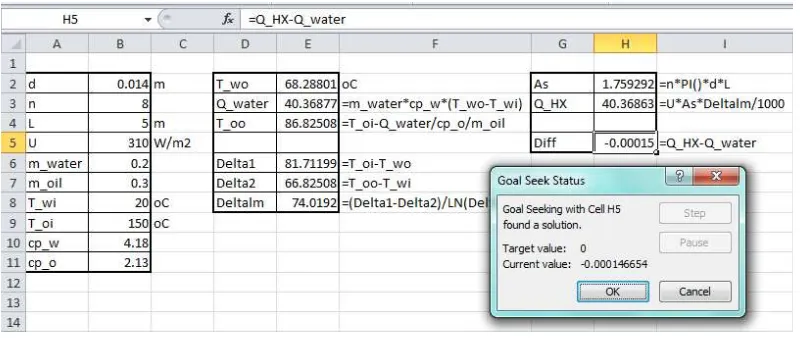
Hot oil at 150°C is to be cooled by water at 20°C in a 1-shell-pass and 8-tube-passes heat exchanger. The length of each tube pass in the heat exchanger is 5 m and the tubes are connected as shown in Figure 1, making one long tube of uniform internal diameter and thickness. The tubes, which are thin-walled with an internal diameter of 1.4 cm, are made of copper and the overall heat transfer coefficient is 310 W/m2·°C. Water flows through the tubes at a rate of 0.2 kg/s, and the oil through the shell at a rate of 0.3 kg/s. It is required to determine the rate of heat transfer in the heat exchanger and the outlet temperatures of the water and the oil.
Figure 1: Schematic for Example 1 (adopted from Cengel and Ghajar [17])
Figure 2: Excel sheet developed for Example 1
The cell E2 stores the guessed value of exit temperature of water (To,w= 90oC), and the cell E4 calculates the corresponding exit temperature for oil (To,o) from Equation (6), which is 58.42oC. As figure 2 shows, the initially guessed exit temperatures lead to a difference (Diff) of -32.12 kJ/s between the heat-transfer rates calculated by Equations (1) and (2). The absolute difference between heat-transfer rates from Equations (1) and (2) should be close to zero at the correct values of To,w and To,o. These values can be found by trial and error, but Excel allows us to find them in a much easier way by using the “Goal-Seek” command. The Goal Seek command is found in the “Data tab”, the “What-If-Analysis” option. Upon selecting Goal Seek, the dialog box shown in Figure 3.a will appear.
(a) (b)
Figure 3: Goal Seek dialog box for Example 1; (a) blank form, (b) filled form
completed dialog box for this example for which the Set cell is H5 that calculates the difference in heat-transfer rates (Diff). The required value for the Set cell is “0” which is to be achieved by changing the value of cell E2 that stores the temperature Tw,o. Pressing the “OK” button will trigger Goal Seek to iterate until the Set cell attains the specified value. Figure 4 shows the solution obtained by Goal Seek.
Figure 4: Goal Seek solution for Example 1
The solution found by Goal Seek is To,w =68.288oC, To,o =86.825oC, and QHX=40.369 kW. Cengel and Ghajar [17] solved the problem by using the ε-NTU method with c=0.764 and NTU=0.854. They found ε=0.47 from chart and, accordingly, obtained To,w =66.8oC and To,o =88.8oC. Since Qmax =83.1 kW, their QHX=39.1 kW. Comparison with the present solution indicates that the precise value for ε is 0.486 and, therefore, the ε-NTU method underestimated the heat-transfer rate by 3.3%.
3. Solution of type-2 and type-3 flow problems
Frictional head loss (hL) in a pipe depends on a number of factors that characterise the pipe itself as well as the velocity and viscosity of the fluid being transported. For a straight pipe with no fittings carrying a viscous Newtonian and incompressible fluid, the Darcy-Weisbach equation states [18]:
g and g the gravitational acceleration constant. For a pipe completely full of fluid, the friction factor (f) is given by the Colebrook-White equation [18]:
iteratively. Therefore, the Colebrook-White equation is usually approximated by the
Practical pipe-flow analyses using the above relationships between the frictional head loss, diameter of the pipe, and the fluid flow rate in the pipe can be divided into three types. A problem of type-1 is that which requires the determination of hL when both the pipe’s diameter and fluid velocity (or flow rate) are known. In this case, Equations (7) and (9) can be used directly to determine the friction head loss. In some problems, referred to as type-2 problems, it is required to determine the flow rate for a specified hL and pipe diameter. Alternatively, if the pipe diameter is to be determined for a given hL and flow rate, then the problem is referred to as a type-3 problem. Both type-2 and type-3 problems require iterative solutions because the friction factor cannot be determined in advance. The following example demonstrates the solution of a type-3 problem using Excel and Goal Seek. The example is adopted from Example 8.4 in Cengel and Cimbala [18].
Example 2: Solution of a type-3 flow problem
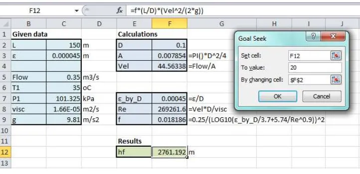
Heated air at 1 atm and 35°C is to be transported in a 150-m-long circular plastic duct (ε=0.000045 m) at a rate of 0.35 m3/s (Figure 5). If the head loss in the duct is not to exceed 20 m, determine the minimum diameter of the duct.
Figure 5: Schematic for Example 2 (adopted from Cengel and Cimbala [18])
The solution can be obtained by calculating the friction head loss at different diameters of the duct and then selecting the diameter that gives the required value of 20 m. An iterative solution proceeds as follows:
1. Select a diameter for the inner pipe (D).
2. Calculate the flow areas of the pipe and velocity of the hot air,
V
V
/
A
. 3. Calculate the Reynolds number in the pipe,Re
VD
/
.4. Calculate the friction factors f from Equation (9). 5. Calculate the friction head loss (hL) from Equation (7). 6. If hL≠20 m, repeat steps 1 to 5.
Figure 6: Excel sheet developed for Example 2
The required duct diameter that gives a head loss of 20 m can be determined by using Goal Seek, which will iterate until the friction head loss attains this value. Figure 6 also shows the completed Goal Seek dialog box for this example. The answer found by Goal Seek is D≥ 0.27 m, which is the same answer given by Cengel and Cimbala [18]. A similar procedure can be used to solve type-2 flow problems by iterating the flow rate instead of the diameter.
4. Determination of the adiabatic flame temperature
The amount of heat released by a combustion reaction, which is called the heat of reaction, heat of combustion, or enthalpy of reaction, is the difference between the total enthalpies of the reactants and the products. This is obtained by applying the first-law of thermodynamics to the combustion process [19]:
is the molar specific enthalpy of the same component which can be calculated from:
i
( 0 is the formation enthalpy of component i at standard condition of 25oC
and 1 atm and hi
~
is the deviation of its specific enthalpy at the relevant state from that at the standard condition [19]. For constant pressure process, hi
~
depends only on the relevant temperature which for reactants is that at the start of the combustion process and for products it is that at the end of the combustion process.
Equation (10) requires the number of moles for both the reactants and products to be known. The combustion equation for a hydrocarbon fuel CαHβ in excess dry air is:
2 2
2 2 2 2combustion
For stoichiometric combustion γ = 1, for lean combustion (with excess air) γ > 1 and for rich combustion (with excess fuel leading to incomplete combustion) γ < 1.
The adiabatic flame temperature (Tf) is the maximum temperature that the combustion products can reach. This temperature occurs in the limiting case of no heat loss to the surroundings (Q =0). From Equation (10): directly from the initial state of the reactants, an iterative process is required in order to determine Tf since the individual products have different enthalpies at the same temperature. Therefore, determination of the adiabatic temperature by hand calculations is both time consuming and inaccurate. However, Tf can easily be determined with Excel and Goal Seek. The following example that demonstrates the procedure is based on Example 4.5 in Pulkrabek [19].
Example 3: Determination of the adiabatic flame temperature
Find the adiabatic flame temperature of isooctane (C8H18) burned with 20% excess dry air. It can be assumed that the reactants are at a temperature of 427oC (700 K) after the compression stroke.
Unlike the two previous examples that dealt with heat-transfer and fluid flow problems, the analysis in this example requires enthalpies of the reactants and products to be evaluated at various temperatures. Therefore, this example requires the use of a suitable property in. In the present analysis, the Thermax property add-in is used. Developed by using Microsoft’s Visual Basic for Applications (VBA), Thermax provides nine groups of user-defined functions for determining the properties of various working fluids. A subset of the add-in that determines the thermodynamic properties of ideal gases and humidified air can be obtained from the author’s page in Researchgate [16]. The procedure for activating the add-in is similar to that of activating the “Solver” add-in, which is explained by the Excel’s help facility under the topic “Add or remove an Excel add-in”.
Figure 7 shows the Excel sheet developed for solving this example by using Goal Seek. To be able to use the same sheet for various fuels and amounts of excess air, it has been generalised for any hydrocarbon fuel with the formula CαHβ and any amount of excess
temperature at Qout = 0. Goal Seek set-up for this example is also shown in Figure 7. The value of Tf determined by Goal Seek was 2475 K while the value determined by Pulkrabek [19] by trial-and-error was 2419 K.
Figure 7: The Excel sheet developed for Example 3 with the relevant Goal seek dialog box
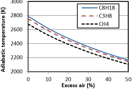
By changing the values of α, β, andγ, the Excel sheet developed for this example can be used to illustrate the effect of excess air on the adiabatic flame temperature from different hydrocarbon fuels. Figure 8 shows the variation of adiabatic flame temperature with the percentage of excess air for
isooctane
(C8H18), propane (C3H8) and methane (CH4) as determined by the present sheet. For all three gases, the figure shows that the adiabatic flame temperature decreases with increasing excess air. The figure also shows that the adiabatic flame temperature for methane is lower than that for propane, which is lower than that forisooctane
. This clearly indicates that the adiabatic flame temperature of a hydrocarbon fuel increases with its molar mass.Figure 8: Effect of excess-air on adiabatic flame temperature
Preparation of the plots shown in Figure 8 requires repeating the same procedure for three fuels and six values of the excess-air parameter (γ). This time-consuming and possible erroneous process can be avoided by using a macro to record the procedure of determining Tf for the first fuel only. The macro can then be utilised to determine Tf for other hydrocarbon fuels after suitably adjusting the values of α and β. Figure 7 shows the macro named “Run” which was used in the preparation of Figure 8.
2000 2200 2400 2600 2800 3000
0 10 20 30 40 50
A
d
iab
atic
te
m
p
e
ratu
re
(K
)
5. Conclusions
The three examples presented in this paper demonstrate the effectiveness of Excel for solving thermal-fluid problems that require iterative solutions via its Goal Seek command. Utilising this capability in the classroom for dealing with such analyses without being distracted by their computational complexities, can accelerate the learning process and improve the students’ problem-solving skills. In this respect, it should be pointed out that Goal Seek starts the iterative process by the initially specified value in the changing cell. Therefore, to obtain the best results from Goal Seek, this initial guess should be physically meaningful and reasonably close to the anticipated solution. That Goal Seek requires value of the Set cell to be entered manually and cannot be automatically read from another cell limits the capability of the tool to single valued optimisation cases. This limitation can be alleviated by using the Solver add-in instead of Goal Seek. Solver enables Excel to perform multi-objective optimisation analyses as well as iterative solutions.
Equipped with a suitable property add-in and Solver, Excel is capable of performing multi-variable optimisation analyses of different types of thermal-fluid systems. The Colebrook-White equation (8) exposes another limitation of Excel that can be solved by developing suitable add-ins or user-defined functions (UDFs) with VBA. If Equation (8) were to be used in solving a type-2 or type-3 problem instead of the explicit equation (9), then two nested iterations would be involved; an inner iteration to determine the friction factor from the implicit equation and an outer iteration to determine the flow rate or pipe diameter. Such nested iterations cannot be handled easily with Excel. In this case, VBA can be used to develop a UDF for solving the implicit equation, leaving the Goal Seek command to perform the main iteration. The developed UDF can also be used to deal with other implicit equations usually met in thermal-fluid analyses, such as the Soave-Redlich-Kwong (SRK) equation [6].
References
[1] Denton, D. (1998), Engineering Education for the 21st Century, Challenges and opportunities. Journal of Engineering Education, Vol. 87, 1998, No. 1, 19-22.
[2] Santana, T. (2007), Computational Tools for Teaching Graduate Courses in Geotechnical Engineering, International Conference on Engineering Education – ICEE 2007, Coimbra, Portugal, September 3 – 7.
[3] The National Science Foundation (NSF), Simulation-based Engineering Science, Revolutionizing Engineering Science through Simulation May 2006, Report of the National Science Foundation Blue Ribbon Panel on Simulation-Based Engineering Science, http://www.nsf.gov/pubs/reports/sbes_final_report.pdf
[4] Dixon, G. W. (2001), Teaching thermodynamics without tables – isn’t it time?,
Proceedings of the 2001 American Society for Engineering Education Annual Conference & Exposition.
[5] F-Chart software, http://www.fchart.com/ees/ (Last accessed April 12, 2016).
[7] Oke, S. A. (2004), Spreadsheet applications in engineering education: A Review, Int. J. Engng Ed. Vol. 20, No. 6, 893-901.
[8] Schumack, M. (2004), Use of a spreadsheet package to demonstrate fundamentals of computational fluid dynamics and heat transfer, Int. J. Engng Ed. Vol. 20, No. 6, 974-983.
[9] Karimi, A. (2009), Using Excel for the thermodynamic analyses of air-standard cycles and combustion processes, ASME 2009 Lake Buena Vista, Florida, USA.
[10] El-Awad, M.M. (2016), Computer-aided thermal design optimisation, International Journal of Innovative Research in Science, Engineering and Technology (IJIRSET), Vol. 5, Issue 1, 1-8.
[11] Ahmadi-Brooghani, Z. (2006), Using Spreadsheets as a Computational Tool in Teaching Mechanical Engineering, Proceedings of the 10th WSEAS International Conference on computers, Vouliagmeni, Athens, Greece, July 13-15, 2006, 305-310.
[12] Lemmon, E.W., Huber, M.L., McLinden, M.O. (2007). NIST Reference Fluid Thermodynamic and Transport Properties— REFPROP Version 8.0, User’s Guide, National Institute of Standards and Technology, Physical and Chemical Properties Division, Boulder, Colorado 80305.
[13] University of Alabama, Mechanical Engineering, Excel for Mechanical Engineering project, http://www.me.ua.edu/excelinme/index.htm. (Last accessed April 7, 2016).
[14] Goodwin, D. G., "TPX: thermodynamic properties for Excel", http://www.tecnun.es/asignaturas/termo/SOFTWARE/TPX/index.html (Last accessed April 12, 2016)
[15] El-Awad, M.M. (2015), A multi-substance add-in for the analyses of thermo-fluid systems using Microsoft Excel, International Journal of Engineering and Applied Sciences (IJEAS), Volume-2, Issue-3, 63-69.
[16] El-Awad, M.M. (2016), https://www.researchgate.net/profile/Mohamed_El-Awad/ contributions, (Last accessed April 12, 2016)
[17] Cengel, Y.A. and Ghajar, A. J. (2011), Heat and Mass Transfer: Fundamentals and Applications. 4th edition, McGraw Hill.
[18]
![Figure 1: Schematic for Example 1 (adopted from Cengel and Ghajar [17])](https://thumb-ap.123doks.com/thumbv2/123dok/3589620.1787100/6.595.224.367.75.205/figure-schematic-example-adopted-cengel-ghajar.webp)
![Figure 5: Schematic for Example 2 (adopted from Cengel and Cimbala [18])](https://thumb-ap.123doks.com/thumbv2/123dok/3589620.1787100/8.595.208.383.411.469/figure-schematic-example-adopted-from-cengel-and-cimbala.webp)