© 2007 Elsevier Science
Neurocomputing 71 (2007) 363–373
Multiplicative updates for non-negative projections
Zhirong Yang
, Jorma Laaksonen
Laboratory of Computer and Information Science, Helsinki University of Technology, P.O. Box 5400, FI-02015 HUT, Espoo, Finland
Received 18 April 2006; received in revised form 20 September 2006; accepted 9 November 2006 Communicated by S. Choi
Available online 20 February 2007
Abstract
We present here how to construct multiplicative update rules for non-negative projections based on Oja’s iterative learning rule. Our method integrates the multiplicative normalization factor into the original additive update rule as an additional term which generally has a roughly opposite direction. As a consequence, the modified additive learning rule can easily be converted to its multiplicative version, which maintains the negativity after each iteration. The derivation of our approach provides a sound interpretation of learning non-negative projection matrices based on iterative multiplicative updates—a kind of Hebbian learning with normalization. A convergence analysis is scratched by interpretating the multiplicative updates as a special case of natural gradient learning. We also demonstrate two application examples of the proposed technique, a non-negative variant of the linear Hebbian networks and a non-negative Fisher discriminant analysis, including its kernel extension. The resulting example algorithms demonstrate interesting properties for data analysis tasks in experiments performed on facial images.
r2007 Elsevier B.V. All rights reserved.
Keywords:Non-negative projection; Multiplicative update; Oja’s rule; Hebbian learning; Matrix factorization
1. Introduction
Projecting high-dimensional input data into a lower-dimensional subspace is a fundamental research topic in signal processing and pattern recognition. Non-negative projection is desired in many real-world applications, for example, for images, spectra, etc., where the original data are non-negative. However, most classical subspace ap-proaches such asprincipal component analysis(PCA) and
Fisher discriminant analysis (FDA), which are solved by
singular value decomposition (SVD), fail to produce the non-negativity property.
Recently, Lee and Seung [12,13] introduced iterative multiplicative updates, which are based on the decomposi-tion of the gradient of given objective funcdecomposi-tion, for non-negative optimizations. They applied the technique to the
non-negative matrix factorization (NMF) which seems to
yield sparse representations. Several variants of NMF such as[5,22,24]have later been proposed, where the original NMF objective function is combined with various regular-ization terms. More recently, Yuan and Oja[23]presented a method calledprojective non-negative matrix factorization
(P-NMF) without any additional terms, but directly derived from the objective function of PCA networks except that the projection was constrained to be non-negative. The simulation results of P-NMF indicate that it can learn highly localized and non-overlapped part-based basis vectors. However, none of the above works provides an explanation why the multiplicative updates can produce sparser and more localized base components.
The multiplicative update rules of the above algorithms are based on decomposition of the gradients of an objective function into positive and negative parts, one as the numerator and the other as the denominator. Nevertheless, such method would fail when the gradient is not naturally expressed in positive and negative parts. Sha et al. [21]
proposed an alternative decomposition of the gradient and applied it to the minimization of a quadratic objective. www.elsevier.com/locate/neucom
0925-2312/$ - see front matterr2007 Elsevier B.V. All rights reserved. doi:10.1016/j.neucom.2006.11.023
Corresponding author.
This method albeit cannot handle the situation where the gradient contains only one positive (negative) term. Furthermore, how to combine orthogonality or quadratic unit norm constraints with this method is still unknown.
In this paper we present a more general technique to reformulate a variety of existing additive learning algo-rithms to their multiplicative versions in order to produce non-negative projections. The derivation is based on Oja’s rule[17]which integrates the normalization factor into the additive update rule. Therefore, our method provides a natural way to form the numerator and denominator in the multiplicative update rule even if external knowledge of gradient decomposition is not available. Another major contribution of our approach is that its derivation also provides a sound interpretation of the non-negative learning based on iterative multiplicative updates—a kind of Hebbian learning with normalization.
We demonstrate applicability of the proposed method for two classical learning algorithms, PCA and FDA, as examples. In the unsupervised PCA learning, our multi-plicative implementation of linear Hebbian networks outperforms the NMF in localized feature extraction, and its derivation provides an interpretation why P-NMF can learn non-overlapped and localized basis vectors. In the supervised FDA learning, our non-negative variant of the
linear discriminant analysis (LDA) can serve as a feature selector and its kernel extension can reveal an underlying factor in the data and be used as a sample selector. The resulting algorithms of the above examples are verified by experiments on facial image analysis with favorable results. The remaining of the paper is organized as follows. First we introduce the basic idea of multiplicative update rules in Section 2. The non-negative projection problem is then formulated in Section 3. In Section 4 we review Oja’s rule and present the technique how to use it in forming the multiplicative update rules. The proposed method is applied in two examples in Section 5: one for unsupervised learning and the other for supervised. The experimental results of the resulting algorithms are presented in Section 6. Finally, conclusions are drawn in Section 7.
2. Multiplicative updates
Suppose there is an algorithm which seeks an m -dimensional solution w that maximizes an objective functionJðwÞ. The conventionaladditive update rule for such a problem is
~
w¼wþggðwÞ, (1)
wherew~is the new value ofw,ga positive learning rate and the functiongðwÞoutputs anm-dimensional vector which represents the learning direction, obtained e.g. from the gradient of the objective function. For notational brevity, we only discuss the learning for vectors in this section, but it is easy to generalize the results to the matrix case, where we will use capital lettersWandG.
The multiplicative update technique first generalizes the common learning rate to different ones for individual dimensions:
~
w¼wþdiagðgÞgðwÞ, (2)
where g is an m-dimensional positive vector. Choosing different learning rates for individual dimensions changes the update direction and hence this method differs from the conventional steepest-gradient approaches in the full real-valued domain.
It has been shown that the following choice of g has particular interesting properties in the constraint of non-negativity (see e.g. [12,21]). Suppose w is non-negatively initialized. If there exists a separation of the learning direction into two positive termsgðwÞ ¼gþgby some
The above multiplicative updatemaintains the non-nega-tivity of w. In addition, wi increases when gþi4gi , i.e.
½gðwÞi40, and decreases if ½gðwÞio0. Thus the
multi-plicative change ofwiindicates how much the direction of that axis conforms to the learning direction. There exists two kinds of stationary points in the iterative use of the multiplicative update rule (3): one satisfies gþ
i ¼gi , i.e. gðwÞ ¼0, which is the same condition for local optima as in the additive updates (1), and the other iswi!0. The latter condition distinguishes the non-negative optimization from conventional ones and yields sparsity inw, which is desired in many applications. Furthermore, unlike steepest gradi-ent or expongradi-ential gradigradi-ent[10], the multiplicative update rule (3) does not require any user-specified learning rates, which facilitates its application.
In most non-negative algorithms that use multiplicative updates (e.g. [13,21,24]), the convergence of the objective has been proven via an auxiliary function. However, such a function depends on particular update rules and sometimes could be difficult to find. Here we present a novel interpretation of multiplicative updates as an optimization using natural gradient [1], which greatly simplifies the convergence analysis of the objective. Define the matrix GðwÞas
with dij the Kronecker delta. The tensor G defines a Riemannian inner product
Henceforth we can obtain the natural gradient ascend
wherez is a positive scalar. Settingz¼1, we obtain the multiplicative update rule (3). Because the natural gradient is known to be the steepest direction in a Riemannian manifold [1], the multiplicative updates form a steepest gradient ascend method inð0;þ1Þmwhich is curved by the tangent of the given objective function. Therefore, the multiplicative update rule (3) guarantees monotonic increase of the objective function ifz¼1 corresponds to a sufficiently small learning step and thus (7) forms a good approximation of the continuous flow in the Riemannian space.
3. Non-negative projection
Subspace projection methods are widely used in signal processing and pattern recognition. An r-dimensional subspace out of Rm can be represented by an mr orthogonal matrixW. In many applications one can write the objective function for selecting the projection matrix in the form
Efg denotes the expectation. For problems where
FðxÞ ¼x, objective (8) can be simplified to Such form covers the objectives of many classical analysis methods such as PCA and Fisher’s LDA. The motivation and neural architecture of (9) is justified in[11]. By setting A¼EfvvTg, we can write the gradient of (9) as
qJðWÞ qW ¼Efvv
T
gW¼AW. (10)
ObviouslyAis a positive semi-definite matrix.
The functionFcan be other thanFðxÞ ¼x. For example, in[8]the log likelihood functionFðxÞ ¼logpðxÞwas used and a variant ofindependent component analysis(ICA) was derived. In that case,A¼EfF0ðkWTvk2ÞvvTgis a negative semi-definite matrix.
In summary, we consider a particular set of additive update rules with the learning direction GðWÞ ¼AW, where A is an mm symmetric matrix. Non-negative projectionrequires that all elements ofWare non-negative. For brevity, we only discuss the case whereAis positive semi-definite. The derivation can easily be modified for the opposite case whereAis negative semi-definite.
4. Oja’s rule in learning non-negative projections
The multiplicative update rule described in Section 2 maintains the non-negativity. However, the gradient of projection objective yields a single term and does not provide any natural way to obtaingþandg(orGþand
G). In this section we present a very simple approach to include an additional term for constructing the multi-plicative update rules if the solution is constrained to be of unitL2-norm or orthogonal.
First let us look at the projection on a one-dimensional subspace. In many optimization problems the objective functionJðwÞis accompanied with the constraint
oðwÞ ¼ ðwTBwÞ1=2
maintains that the newwstill satisfies (11) sinceoðbwÞ ¼
boðwÞfor a scalarb.
One may try to combine the two update steps (1) and (12) into a single step version. The normalization factor ðoðwÞÞ1can be expressed using Taylor expansion as
ðoðwÞÞ~ 1¼ ðw þggÞTBðwþggÞ1=2
¼1þgðwTBgþgTBwÞ þOðg2Þ1=2
11
2gðw
TBgþgTBwÞ. ð13Þ
Hereg¼gðwÞfor brevity and the final step is obtained by dropping all terms ofOðg2Þor higher orders. Inserting this result and (1) into (12), we obtain the following Oja’s single-step update rule[17]:
wnewwþ1
2gð2gww TBg
wgTBwÞ, (14)
where again the terms ofOðg2Þhave been dropped. Now setting gðwÞ ¼Aw, we obtain a possible decom-position ofgðwÞinto two non-negative parts as
gðwÞ ¼Aw¼AþwAw, (15)
The simple update rule
wnewi ¼wi
is non-negative, i.e. A¼0. As an alternative, we here
propose to substitutegfrom (15) into (14) and then obtain
wnewwþ1 2gð2A
þw
2AwwwTBAwwwTABwÞ.
(19)
Supposewis initialized with values inð0;1Þand fulfills (11). All terms without their leading sign in the right side of (19) are then positive ifwTðBAþABÞw40 for all positive w.
This condition defines the convexity of the solution subspace and is satisfied whenBAþABis positive definite. Verifying such positive definity can easily be done before the iterative learning.
We can then apply the generalization technique de-scribed in Section 2 and obtain the following multiplicative update rule:
SinceBis symmetric, (20) can be further simplified to
wnewi ¼wi
½Aþwi
½Aw
iþ ½wwTBAwi
(21)
because in that case
wTBAw¼ ðwTBAwÞT¼wTATBTw¼wTABw. (22)
The original Oja’s rule for a single vector has been generalized to the matrix case [18]. It combines the following additive learning rule and normalization steps:
~
W¼WþgGðWÞ, (23)
Wnew¼Wð~ XðWÞÞ~ 1, (24)
whereWandGaremrmatrices and
XðWÞ ¼I (25)
is the optimization constraint in the matrix case. If
XðWÞ ¼ ðWTWÞ1=2, the normalization factor can be
with similar derivation as in (13). Inserting (26) and (23) into (24), we obtain
WnewWþ1
2gð2GWW
TGWGTWÞ. (27)
By again applying the generalization on g and inserting G¼AW, we can get the following multiplicative update rule:
Our method is suitable for problems with the constraint of the formWTW¼IorwTBw¼1, but generally it does not work for WTBW¼I if BaI. This is because such constraint ofB-uncorrelatedness is probably overwhelmed by the non-negative learning which tends to yield high orthogonality.
If one only considers the projection on the Stiefel manifold (i.e. WTW¼I), a more straightforward deriva-tion can be obtained by using the natural gradient. Given a learning direction G¼AW, the natural gradient ascend update is[16]
Wnewnat ¼WþgðGWGTWÞ. (29)
Substituting A¼AþA and applying the reforming technique on g, we obtain the same multiplicative update rule (28). This is not surprising because Oja’s rule and natural gradient are two essentially equivalent optimization methods on the Stiefel manifold except that the former is based on the ordinary Euclidean metric while the latter on a canonical Riemannian metric[4].
5. Examples
In this section, we apply the above reforming technique to two known projection methods, PCA and LDA. Before presenting the details, it should be emphasized that we are not aiming at producing new algorithms to replace the existing ones for reconstruction or classification. Instead, the main purpose of these examples is to demonstrate the applicability of the technique described in the previous section and to help readers get more insight in the reforming procedure.
5.1. Non-negative linear Hebbian networks
Using multiplicative updates for non-negative optimiza-tion stems from the NMF proposed by Lee and Seung[12]. Given an mn non-negative input matrix V where columns are the input samples, NMF seeks two non-negative matricesWandHwhich maximizes the following objective:
JNMFðW;HÞ ¼ kVWHkF. (30)
Herek kFis the Frobenius matrix norm, defined as
kQkF¼X
ij
Q2ij (31)
for a matrixQ. The authors of[12]derived the following multiplicative update rules of NMF:
Wnew
optimization problem:
minimize
WX0 JP-NMFðWÞ ¼ kVWW T
VkF. (34)
That is, P-NMF replaces the matrixH with WTVin the objective function. This change makes P-NMF also a variant of PCA whose objective is same as that of P-NMF except the non-negative constraint. The unconstrained gradient ofJP-NMFðWÞis given by
qJP-NMFðWÞ
upon which the authors of [23] obtained the following multiplicative update rule using the technique in Section 2:
Wnew
Similar to NMF, P-NMF is not the best method to minimize the reconstruction error. Instead, it focuses in training orthogonal basis vectors. The simulation results in
[23] showed that P-NMF is capable of extracting highly localized, sparse, and non-overlapped part-based features. However, there is little explanation about this phenomenon in[23].
In this example we employ the reforming technique of the previous section to derive a new multiplicative update rule, named Non-negative linear Hebbian network
(NLHN), for finding the non-negative projection. Given an
m-dimensional non-negative input vectorv, we define the learning direction by the simplest linear Hebbian learning rule, i.e. the product of the input and the output of a linear network:
This result is tightly connected to the PCA approach because the corresponding additive update rule
Wnew¼WþgðvvTWWWTvvTWÞ (39)
is a neural network implementation of PCA [18], which results in a set of eigenvectors for the largest eigenvalues of
EfðvEfvgÞðvEfvgÞTg. However, these eigenvectors and
the principal components of data found by PCA are not necessarily non-negative.
In addition to the on-line learning rule (38), we can also use its batch version
Wnewij ¼Wij
We can see that NLHN bridges NMF and P-NMF. While the latter replaces H with WTV in the NMF objective function (30), NLHN applies similar replacement in the update rule (32) of NMF. In addition, NLHN can be considered as a slight variant of P-NMF. To see this, let us decompose (35) into two parts
qJP-NMFðWÞ little effect in learning the principal directions[9]. Thus, by dropping Gð2Þ, we obtain the same multipli-cative update rule as (40) based on Gð1Þ. Unlike other variants of NMF such as[5,14,22], NLHN does not require any additional regularization terms. This holds also for P-NMF.
The major novelty of NLHN does not lie in its performance as we have shown that it is essentially the same as P-NMF. We will also show by experiments in Section 6.2 that NLHN behaves very similarly to P-NMF. However, the interpretation of P-NMF as a variant of simple Hebbian learning with normalization helps us understand the underlying reason that P-NMF and NLHN are able to learn more localized and non-overlapped parts of the input samples.
As we know, iteratively applying the same Hebbian learning rule will result in that the winning neuron is repeatedly enhanced, and the normalization forces only one neuron to win all energy from the objective function
[7]. In our case, this means that only one entry of each row ofW will finally remain non-zero and the others will be squeezed to zero. That is, the normalized Hebbian learning is the underlying cause of the implicit orthogonalization. Furthermore, notice that two non-negative vectors are orthogonal if and only if their non-zero parts are not overlapped.
Then why can P-NMF or NLHN produce localized representations? To see this, one should first notice that the objectives of P-NMF and NLHN are essentially the same if Wis orthonormal. Therefore, let us only consider here the objective of NLHN,JNLHNðWÞ ¼EfkWTvk2g, which can be interpreted as the mean correlation between projected vectors. In many applications, e.g. facial images, the correlation often takes place in neighboring pixels or symmetric parts. That is why P-NMF or NLHN can extract the correlated facial parts such as lips and eye brows, etc.
We can further deduce the generative model of P-NMF or NLHN. Assume each observationv is composed of r
non-overlapped parts, i.e.v¼Pr
p¼1vp. In the context of
orthogonality, P-NMF models each partvpby the scaling of a basis vectorwpplus a noise vectorep:
vp¼apwpþep. (42)
If the basis vectors are normalized so that wT
pwq¼1
of this part is
The norm of the reconstruction error is therefore bounded by
vp if 2-norm is used. Similar bounds can be derived for other types of norms. In words,wpwTpvp reconstructsvp well if the noise level ep is small enough. According to this model, P-NMF or NLHN can potentially be applied to signal processing problems where the global signals can be divided into several parts and for each part the observations mainly distribute along a straight line modeled byapwp. This is closely related to Oja’s PCA subspace rule [18], which finds the direction of the largest variation, except that the straight line found by P-NMF or NLHN has to pass through the origin. It is important to notice that we analyze the forces of orthogonality and locality separately only for simplicity. Actually either P-NMF or NLHN implements them in the same multiplicative updates and these forces work con-currently to attain both goals during the learning.
5.2. Non-negative FDA
Given a set of non-negative multivariate samples xðiÞ,
i¼1;. . .;n, from the vector spaceRm, where the index of each sample is assigned to one ofQclasses,FisherLDA finds the directionwfor the following optimization problem:
maximize
HereSBis thebetween classes scatter matrixandSWis the
within classes scatter matrix, defined as SB¼1
wherencandIcare the number and indices of the samples in classc, and
and notice that thetotal scatter matrixST¼SBþSW, the LDA problem can be reformulated as
maximize
and hence becomes a particular case of (9).
The common solution of LDA is to attach the con-straint (46) to the objective function with a Lagrange multiplier, and then solve theKarush–Kuhn–Tucker(KKT) equation by SVD. This approach, however, fails to produce the non-negativity of w. To overcome this, we apply the multiplicative update technique described in Section 4 and obtain the following novel alternative method here named non-negative linear discriminant analysis(NLDA).
We start from the steepest-gradient learning:
gðwÞ ¼qð
with the elements ofwinitialized with random values from ð0;1Þ and wTSWw¼1 fulfilled. Here Sþ
B and S
B are determined by (16). If the symmetric matrix SWSBþ
ðSWSBÞT¼SWSBþSBSWis positive definite, then
wTS
That is, all terms on the right side of (55) are positive and so is the newwafter each iteration. Moreover, notice that NLDA does not require matrix inversion of SW, an operation which is computationally expensive and possibly leads to singular problems.
2Cg4medianfxjjxj2C¯g, we transform the original data
by
xj Yjxj, (57)
whereYjis the known upper bound of thejth dimension. After such flipping, for each dimension j there exists a threshold yj which is larger than more than half of the samples ofCand smaller than more than half of the samples of C¯. That is, the classCmainly distributes the inner part closer to the origin while C¯ distributes the outer part farther from the origin. Projecting the samples to the direction obtained by (55) will thus yield better discrimination.
The above non-negative discriminant analysis can be extended to non-linear case by using the kernel technique. Let U be a mapping from Rm toF, which is implicitly defined by a kernel functionkðx;yÞ ¼kðy;xÞ ¼UðxÞT
UðyÞ.
kernel Fisher discriminant analysis(KFDA)[2,15] finds a directionwin the mapped spaceF, which is the solution of the optimization problem
B andSUWare the corresponding between-class and within-class scatter matrices. We use hereSU
T¼SUBþSUW instead ofSUWfor simplification, but it is easy to see that the problems are equivalent. From the theory of reproducing kernels[20]we know that any solutionw2Fmust lie in the span of all training samples inF. That is, there exists an expansion forwof the form
w¼X
n
i¼1
aiUðxðiÞÞ. (60)
It has been shown[2]that by substituting (60) into (58) and (59), the unconstrained KFDA can be expressed as
maximize
The matrices K and U are symmetric and all their elements are non-negative. We can obtain the following multiplicative update rule for novel non-negative kernel Fisher discriminant analysis (NKFDA) by setting A¼ Aþ¼KUKandB¼KKin (21):
This formulation has the extra advantage that the resulting elements ofa indicate the contribution of their respective samples in forming the discriminative projection. This is conducive to selecting among the samples and revealing the underlying factor in the data even if we only use the simple linear kernel, i.e.UðxÞ ¼x.
6. Experiments
We demonstrate here the empirical results of the non-negative algorithms presented in Sections 5.1 and 5.2 when applied for processing of facial images. Before proceeding to details, it should be emphasized that the goal of the non-negative version of a given algorithm usually differs from the original one. The resulting objective value of a non-negative algorithm generally is not as good as that of its unconstrained counterpart. However, readers should be aware of that data analysis is not restricted to reconstruction or classification and that non-negative learning can bring us novel insights in the data.
6.1. Data
We have used the FERET database of facial images[19]. After face segmentation, 2409 frontal images (poses ‘‘fa’’ and ‘‘fb’’) of 867 subjects were stored in the data-base for the experiments. We obtained the coordinates of the eyes from the ground truth data of FERET collection, with which we calibrated the head rotation so that all faces are upright. Afterwards, all face boxes were normalized to the size of 3232, with fixed locations for the left eye (26,9) and the right eye (7,9). Each image was reshaped to a 1024-dimensional vector by column-wise concatenation.
Another database we used is the UND database (collection B) [6], which contains 33,247 frontal facial images. We applied the same preprocessing procedure to the UND images as to the FERET database.
6.2. Non-negative linear Hebbian networks
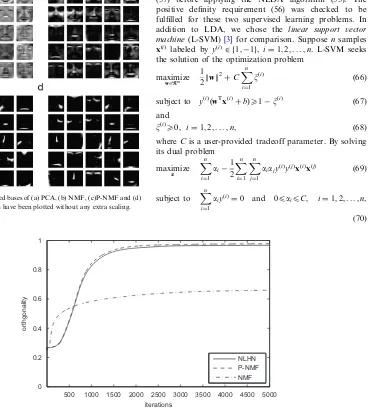
First we compared four unsupervised methods: PCA, NMF [12], P-NMF [23] and NLHN (40) for encoding the faces. The resulting basis images are shown in Fig. 1. It can be seen that the PCA bases are holistic and it is hard to identify the parts that compose a face. NMF yields partially localized features of a face, but some of them are still heavily over-lapped. P-NMF and NLHN are able to extract the highly sparse, local and non-overlapped parts of the face, for example the nose and the eyebrows. The major difference between P-NMF and NLHN is only the order of the basis vectors.
Orthogonality is of main interests for part-based learning methods because that property leads to non-overlapped parts and localized representations as discussed in Section 5.1. Suppose the normalized inner product between two basis vectorswiandwjis
Rij¼ wT
iwj
kwikkwjk
Then the orthogonality of anmrbasisW¼ ½w1;. . .;wr can be quantified by the followingr-measurement:
r¼1
P
iajRij
rðr1Þ (65)
so thatr2 ½0;1. Largerr’s indicate higher orthogonality and
rreaches 1 when the columns ofWare completely orthogonal.
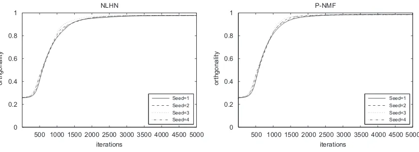
Fig. 2shows the evolution ofr’s by using NMF, NLHN and P-NMF with dimensionsm¼1024 andr¼25. NMF converges to a local minimum withr¼0:63, while NLHN
and P-NMF learnWwithr¼0:97 and 0.98, respectively, after 5000 iterations. We also trained NLHN and P-NMF with different random seeds for the initial values ofWand the results are shown inFig. 3. It can be seen that both methods converge with very similar curves. That is, NLHN behaves very similarly to P-NMF in attaining high orthogonality, and being not sensitive to the initial values.
6.3. Non-negative linear discriminant analysis
Next, we demonstrate the application of the linear supervised non-negative learning in discriminating whether the person in a given image has mustache and whether he or she is wearing glasses. The data were preprocessed by (57) before applying the NLDA algorithm (55). The positive definity requirement (56) was checked to be fulfilled for these two supervised learning problems. In addition to LDA, we chose the linear support vector machine(L-SVM)[3] for comparison. Supposensamples xðiÞ labeled by yðiÞ2 f1;1g, i¼1;2;. . .;n. L-SVM seeks
the solution of the optimization problem
maximize w2Rm
1 2kwk
2þCXn
i¼1
xðiÞ (66)
subject to yðiÞðwTxðiÞþbÞX1xðiÞ
(67)
and
xðiÞX0; i¼1;2;. . .;n, (68)
whereCis a user-provided tradeoff parameter. By solving its dual problem
maximize a
Xn
i¼1
ai 1 2
Xn
i¼1
Xn
j¼1
aiajyðiÞyðjÞxðiÞxðjÞ (69)
subject to X n
i¼1
aiyðiÞ¼0 and 0paipC; i¼1;2;. . .;n, (70)
500 1000 1500 2000 2500 3000 3500 4000 4500 5000 0
0.2 0.4 0.6 0.8 1
iterations
orthgonality
NLHN P-NMF NMF
Fig. 2. rvalues of NLHN, P-NMF and NMF with 25 basis vectors and 1024-dimensional data. Fig. 1. The top 25 learned bases of (a) PCA, (b) NMF, (c)P-NMF and (d)
one obtains the optimalw¼Pn
i¼1aiyðiÞxðiÞwith respect to the givenC.
Fig. 4displays the respective resulting LDA, L-SVM and NLDA projection vectors as images. It is hard to tell from the LDA projection vector in which dimensions of the input samples are most relevant for discriminating mus-tache or glasses. Such poor filters are probably caused by overfitting because LDA may require large amount of data to approximate the within-class covariance bySWbut this becomes especially difficult for high-dimensional problems. The filter images of L-SVM are slightly better than those of LDA. A distinguishing part can roughly be perceived between the eyes. Nevertheless there are still many irrelevant points found by L-SVM. In contrast, the NLDA training clearly extract the relevant parts, as shown by the brightest pixels in the rightmost images in Fig. 4. Such results conform well to the human intuition in this task.
Next we compared the above methods in classification where the training data were the FERET database and test data were the UND database. The compared methods try
to classify whether the person in the image wears glasses or not because both data sets contain this kind of ground truth data. (Unfortunately the UND database does not include such data on mustache.) The results are shown in
Table 1, from which we can see that LDA performs best in classifying the training samples, but very poorly for the new data outside of the training set.
L-SVM requires choice of the tradeoff parameterC. To our knowledge, there are no efficient and automatic methods for obtaining its optimal value. In this experiment we trained different L-SVMs with the tradeoff parameter in f0:01;0:03;0:1;0:3;1;3;10;30;100g and it turned out that the one with 0:03 performed best in fivefold cross-validations. Using this value, we trained an L-SVM with all training data and ran the classification on the test data. The result shows that L-SVM generalizes better than LDA, but the test error rate is still much higher than the training one, which is possibly because of some overfitting dimensions in the L-SVM filter. Higher classification accuracy could be obtained by applying non-linear kernels. This, however, requires more effort to choose among kernels and associated kernel parameters, which is beyond the scope of this paper.
The last column ofTable 1shows that NLDA performed even better than L-SVM in classifying the test samples. This is possibly because of the variation between the two databases. In such a case, the NLDA filter, which resembles more our prior knowledge, tends to be more reliable.
500 1000 1500 2000 2500 3000 3500 4000 4500 5000 0
0.2 0.4 0.6 0.8 1
iterations
orthgonality
NLHN
Seed=1 Seed=2 Seed=3 Seed=4
500 1000 1500 2000 2500 3000 3500 4000 4500 5000 0
0.2 0.4 0.6 0.8 1
iterations
orthgonality
P-NMF
Seed=1 Seed=2 Seed=3 Seed=4
Fig. 3.rvalues of NLHN and P-NMF with different random seeds.
Fig. 4. Images of the projection vector for discriminating glasses (the first row) and mustache (the second row). The methods used from left to right are LDA, L-SVM, NLDA.
Table 1
Equal error rates(EERs) of training data (FERET) and test data (UND) in classification of glasses versus no glasses
LDA L-SVM NLDA
FERET (%) 0.98 11.69 17.54
6.4. Non-negative kernel Fisher discriminant analysis
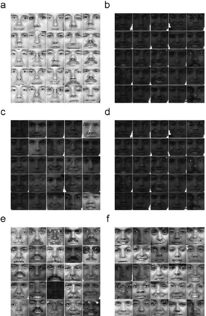
Furthermore, we tested the function of NKFDA (63) that ranks the training samples by their contribution to the projection. We used only the linear kernel here because of its simplicity. After training of NKFDA on the FERET data labeled whether the subject has mustache, we sorted the training samples in the order of their respective values ofai.
The top 25 faces and the bottom 25 faces are shown in
Figs. 5(a) and (b), respectively. It can be clearly seen that the most important factor is the lighting condition. This could be expected because we are using well-aligned facial images of front-pose and neutral expression. Therefore the most significant noise here can be assumed to be variation in lighting. In addition, this order agrees with the common perception of humans, where the lighting that provides enough contrast helps in discriminating semantic classes.
For comparison, we display the ordered results of two compared methods.Figs. 5(c) and (d) show the top 25 and
bottom 25 faces of KFDA, respectively. Because the coefficients produced by KFDA are not necessarily non-negative, we sorted the faces by their absolute values. The bottom images look similar to those obtained by NKFDA. That is, darker images that provide poor contrast contribute least to the discrimination. However, it is hard to find a common condition or easy interpretation for the KFDA ranking of the top faces.
The resulting top and bottom facial images of L-SVM are shown inFigs. 5(e) and (f). As we know, the samples with non-zero coefficients are support vectors, i.e. those around the classification boundary, which explains the top images ranked by L-SVM. On the other hand, the samples far away from the boundary will be associated with zero coefficients. In this case, they are mostly typical non-mustache faces shown inFig. 5(f).
7. Conclusions
We presented a technique how to construct multi-plicative updates for learning non-negative projections based on Oja’s rule, including two examples of its application to reforming the conventional PCA and FDA to their non-negative variants. In the experiments on facial images, the non-negative projections learned by using the novel iterative update rules have demonstrated interesting properties for data analysis tasks in and beyond recon-struction and classification.
It is still a challenging and open problem to mathema-tically prove the convergence of orthogonality. The deri-vation of our method provides a possible interpretation of the multiplicative updates. The numerator part favors the learning in the original direction while the denominator part is mainly responsible for the normalization constraint. These two forces work together to steer the learning towards a local optimum. Iteratively applying such a multiplicative update rule yields one of the two sorts of stationarity in each dimension, one approaching zero and the other reaching the natural upper bound. Note that none of the elements can approach infinity because of the normalization. In the terms of neural networks, this can be interpreted as a competition between the elements, both within a neuron and across the neurons. In the matrix case, more than one neuron compete for the energy from the objective function and only one of them wins all over the others, which leads to high orthogonality between the learned basis vectors.
References
[1] S. Amari, Natural gradient works efficiently in learning, Neural Comput. 10 (2) (1998) 251–276.
[2] G. Baudat, F. Anouar, Generalized discriminant analysis using a kernel approach, Neural Comput. 12 (10) (2000) 2385–2404. [3] N. Cristianini, J. Shawe-Taylor, An Introduction to Support Vector
Machines, Cambridge University Press, Cambridge, 2000. [4] A. Edelman, The geometry of algorithms with orthogonality
constraints, SIAM J. Matrix Anal. Appl. 20 (2) (1998) 303–353. Fig. 5. The images with: (a) largest and (b) smallest values inatrained by
[5] T. Feng, S.Z. Li, H.Y. Shum, H.J. Zhang, Local non-negative matrix factorization as a visual representation, in: Proceedings, The Second International Conference on Development and Learning, 2002, pp. 178–183.
[6] P.J. Flynn, K.W. Bowyer, P.J. Phillips, Assessment of time dependency in face recognition: an initial study, Audio- and Video-Based Biometric Person Authentication, 2003, pp. 44–51. [7] S. Haykin, Neural Networks—A Comprehensive Foundation, second
ed., Prentice-Hall, Englewood Cliffs, NJ, 1998.
[8] A. Hyva¨rinen, P. Hoyer, Emergence of phase- and shift-invariant features by decomposition of natural images into independent feature subspaces, Neural Comput. 12 (7) (2000) 1705–1720.
[9] J. Karhunen, J. Joutsensalo, Generalizations of principal component analysis, optimization problems, and neural networks, Neural Net-works 8 (4) (1995) 549–562.
[10] J. Kivinen, M. Warmuth, Exponentiated gradient versus gradient descent for linear predictors, Inf. Comput. 132 (1) (1997) 1–63. [11] T. Kohonen, Emergence of invariant-feature detectors in the
adaptive-subspace self-organizing map, Biol. Cybern. 75 (1996) 281–291. [12] D.D. Lee, H.S. Seung, Learning the parts of objects by non-negative
matrix factorization, Nature 401 (1999) 788–791.
[13] D.D. Lee, H.S. Seung, Algorithms for non-negative matrix factoriza-tion, in: NIPS, 2000, pp. 556–562.
[14] W. Liu, N. Zheng, X. Lu, Non-negative matrix factorization for visual coding, in: Proceedings of IEEE International Conference on Acoustics, Speech, and Signal Processing (ICASSP 2003), vol. 3, 2003, pp. 293–296.
[15] S. Mika, G. Rtsch, J. Weston, B. Scho¨lkopf, K.-R. Mller, Fisher discriminant analysis with kernels, Neural Networks Signal Process. IX (1999) 41–48.
[16] Y. Nishimori, S. Akaho, Learning algorithms utilizing quasi-geodesic flows on the Stiefel manifold, Neurocomputing 67 (2005) 106–135. [17] E. Oja, A simplified neuron model as a principal component analyzer,
J. Math. Biol. 15 (1982) 267–273.
[18] E. Oja, Principal components, minor components, and linear neural networks, Neural Networks 5 (1992) 927–935.
[19] P.J. Phillips, H. Moon, S.A. Rizvi, P.J. Rauss, The FERET evaluation methodology for face recognition algorithms, IEEE Trans. Pattern Anal. Mach. Intell. 22 (2000) 1090–1104.
[20] B. Scho¨lkopf, A. Smola, Learning with Kernels, MIT Press, Cambridge, MA, 2002.
[21] F. Sha, L.K. Saul, D.D. Lee, Multiplicative updates for large margin classifiers, in: COLT, 2003, pp. 188–202.
[22] B.W. Xu, J.J. Lu, G.S. Huang, A constrained non-negative matrix factorization in information retrieval, in: Proceedings of the 2003 IEEE International Conference on Information Reuse and Integra-tion (IRI2003), 2003, pp. 273–277.
[23] Z. Yuan, E. Oja, Projective nonnegative matrix factorization for image compression and feature extraction, in: Proceedings of 14th Scandinavian Conference on Image Analysis (SCIA 2005), Joensuu, Finland, June 2005, pp. 333–342.
[24] S. Zafeiriou, A. Tefas, I. Buciu, I. Pitas, Class-specific discriminant non-negative matrix factorization for frontal face verification, in: Proceedings of Third International Conference on Advances in Pattern Recognition (ICAPR 2005), vol. 2, 2005, pp. 206–215.
Zhirong Yangreceived his Bachelor and Master degrees in Computer Science from Sun Yat-Sen University, Guangzhou, China, in 1999 and 2002, respectively. Presently he is a doctoral candidate at the Computer and Information Science La-boratory in Helsinki University of Technology. His research interests include machine learning, pattern recognition, computer vision, and multi-media retrieval.