Full Terms & Conditions of access and use can be found at
http://www.tandfonline.com/action/journalInformation?journalCode=ubes20
Download by: [Universitas Maritim Raja Ali Haji] Date: 12 January 2016, At: 17:56
Journal of Business & Economic Statistics
ISSN: 0735-0015 (Print) 1537-2707 (Online) Journal homepage: http://www.tandfonline.com/loi/ubes20
Who Does Not Respond in the Household
Expenditure Survey
Edna Schechtman, Shlomo Yitzhaki & Yevgeny Artsev
To cite this article: Edna Schechtman, Shlomo Yitzhaki & Yevgeny Artsev (2008) Who Does Not
Respond in the Household Expenditure Survey, Journal of Business & Economic Statistics, 26:3, 329-344, DOI: 10.1198/00
To link to this article: http://dx.doi.org/10.1198/00
Published online: 01 Jan 2012.
Submit your article to this journal
Article views: 55
Who Does Not Respond in the Household
Expenditure Survey: An Exercise in
Extended Gini Regressions
Edna S
CHECHTMANDepartment of Industrial Engineering and Management, Ben-Gurion University, Beer Sheva, Israel (ednas@bgu.ac.il)
Shlomo Y
ITZHAKIHebrew University and Central Bureau of Statistics, Jerusalem 95464, Israel (Shlomo.yitzhaki@huji.ac.il)
Yevgeny A
RTSEVCentral Bureau of Statistics, Jerusalem 95464, Israel (yevgenya@cbs.gov.il)
A nonparametric multiple regression method, based on the extended Gini that depends on one parameter, ν, is investigated. The parameterνenables production of infinite alternative linear approximations to the regression curve which differ in the weighting schemes applied to the slopes of the curve. The method allows the investigator to stress different sections of one independent variable while keeping the treatment of the other independent variables intact. As an application we investigate nonresponse patterns in a survey of household expenditures to learn about the relationship between nonresponse and income. The empirical results show that the higher the income, the higher the response rate, and the larger the household, the higher the response rate. The Arab population tends to respond more than the Jewish one, whereas the ultrareligious group tends to respond less than the rest of the population. The implications on the bias in the estimates are discussed.
KEY WORDS: Extended Gini; Nonresponse; Regression.
1. INTRODUCTION
The purpose of this article is to present a new, nonparametric multiple regression method, based on the extended Gini (EG) measures of dispersion, for investigating the curvature of a re-gression curve. The method is capable of estimating a series of linear approximations of the regression curve, allowing the investigator to stress different sections along the range of one independent variable, while keeping the weighting scheme of other independent variables intact. This property enables the researcher to learn whether the conditional regression curve is linear, convex, or concave in one independent variable, given the weighting scheme applied to the slopes of the other inde-pendent variables. The method is based on the extended Gini family that depends on one parameter,ν. The choice of this pa-rameter enables the user to produce infinite alternative estima-tors of the regression curve. The main purpose of the method from an econometric point of view is descriptive. One major advantage is that it can treat each independent variable individ-ually, concentrating on the (conditional) relationship between the dependent variable and one independent variable, given the other independent variables. All regressions rely on all obser-vations, eliminating the need to arbitrarily define windows, or omit observations (but there is arbitrariness in the choice ofν). The drawback of the EG approach is that it is not based on a di-rect derivation as are other derivative estimators (Powell, Stock, and Stoker 1989).
The methodology is illustrated by investigating the tendency not to respond to questionnaires on finances of the household in official surveys. The common wisdom with respect to this issue is that either or both rich and poor people tend to respond less than ordinary people. Since we have no firm priors with
respect to the kind of relationship we expect to see, the need for a nonparametric method that can analyze the data arises.
The main conclusion of the empirical application is that non-response to the survey of family expenditures in Israel is a decreasing convex function of income, and almost reaches a plateau when high-income groups are stressed. Nonresponse tends to be negatively related to household size. The nonre-sponse rate differs among ethnic groups: the Arab population shows below-average nonresponse rate, while the ultrareligious Jewish group has above-average nonresponse rate. This result holds even when the response rate is adjusted for income and household size.
Because the estimators in this article are based on the sam-ple’s analogs of the population parameters, we will use capital letters to represent population parameters and lowercase letters to represent the estimators.
The structure of the article is the following: Section 2 presents the nonparametric regression coefficients in the sim-ple regression case. Section 3 extends it to a multisim-ple regres-sion framework, and Section 4 presents the estimators and their standard errors. Readers who are not interested in the exact derivation of the estimates and their standard errors can skip the fourth section. Section 5 presents the data and the research question, the sixth section presents the empirical results, and the seventh evaluates the implication of nonresponse on mea-surement of inequality. Section 8 concludes.
© 2008 American Statistical Association Journal of Business & Economic Statistics July 2008, Vol. 26, No. 3 DOI 10.1198/00 329
2. SIMPLE REGRESSION CASE
Let(Y,X)be a bivariate random variable with expected val-ues μY andμX and finite variances σY2 andσX2, respectively,
and letg(x)=E{Y|X=x}be the regression curve. The error term at(Yi,Xi)is defined as the deviation of Yi from a linear
approximation α+βXi, that is, εi =Yi−α−βXi, where α
andβ are parameters to be defined later. Aside from the prop-erties implied by the assumptions on(Xi,Yi), no additional
as-sumptions are imposed on the error term, and no structure is imposed on the regression curve. In particular, this means that E{ε|X=x} =g(x)−α−βx, which is equal to zero for all val-ues ofxonly ifg(x)is a linear function ofx.
We are interested in estimating a linear approximation to the regression curve,g(x). We start with the parameter represent-ing the slope, β, and only later deal with the constant term. The parameter representing the slope of the linear approxima-tion of the regression curve will be referred to as the EGRC (extended Gini regression coefficient). The slope will be de-fined as a weighted average of the derivatives ofg(x), with the weights being derived from the extended Gini variability in-dex. In some sense, the approach in this article can be viewed as similar to the one presented in Angrist, Chernozhukov, and Fernándaz-Val (2004), who analyzed the linear approximation of a misspecified model in a quantile regression approach.
The extended Gini variability index is a member of a family of indices defined by
G(X, ν)= −(ν+1)COV
X,[1−F(X)]ν
, ν >−1, ν=0. By determining ν, the investigator introduces his preference concerning the measurement of variability of the independent variable. The role ofν in the extended Gini variability index is to reflect the investigator’s attitude toward variability. The higherν is, the more stress is put on the lower portion of the distribution of the independent variable. In the extreme case (ν→ ∞), the investigator cares only about the lowest part of the cumulative distribution, as if he is guided by the max– min criterion. Ifν=1, then the investigator measures variabil-ity according to Gini’s mean difference, implying a symmetric weighting scheme around the median. Ifν→0, the investigator does not care about variability; the range−1≤ν <0 reflects giving higher weights to the upper side of the distribution of the independent variable, whileν→ −1 implies an investigator whose attitude to variability follows the max–max strategy, that is, caring about variability around the highest part of the distri-bution only. It is worth noting that when−1≤ν <0, the index of variability is negative. (See Donaldson and Weymark 1983; Yitzhaki 1983; and Chakravarty 1988, chap. 3, pp. 82–102, for description of the properties of the extended Gini index. Gar-ner 1993, Lerman and Yitzhaki 1994, and Wodon and Yitzhaki 2002 are examples of its decomposition and use in welfare eco-nomics; see Araar and Duclos 2003 for a possible extension; see Davidson and Duclos 1997 for statistical inference, and Millimet and Slottje 2002 for an application in environmen-tal economics.) However, in the above-mentioned literature, the parameter is restricted toν >0. Schechtman and Yitzhaki (1987, 1999, 2003) defined and investigated the properties of the equivalents of the covariance and the correlation. Yitzhaki and Schechtman (2005) offered a survey of the properties of
the EG family and, in particular, showed the metric that leads to the EG. The decomposition of the extended Gini of a sum of random variables into the contributions of the extended Gini’s of the individual random variables and the (equivalents of) correlations among them can also be found there. Olkin and Yitzhaki (1992) defined the simple Gini regression coefficients and investigated their properties. Serfling and Xiao (2006) de-fined and investigated the properties of multivariateL-moments which include the EG moments as a special case.
It is worth mentioning that the parameters of the simple re-gression have been already in use for almost two decades in two major economic fields: welfare economics and risk aversion. In these fields the investigator who cares about the effect of a pol-icy on the margin is interested in a weighted average of slopes between adjacent observations, weighted by the marginal util-ity (or the social evaluation of the marginal utilutil-ity in welfare economics) of income on a curve. There is no need, from the economic model point of view, to assume or to require linearity, and the assumption of linearity is introduced in the estimation process by the econometrician (who may be the same person). In those cases the determination of the weighting scheme (i.e., the choice ofν) should be determined by the social views (or risk aversion) that guide the investigator. For a survey on the applications in the area of welfare economics, see Wodon and Yitzhaki (2002), whereas the applications in finance are demon-strated in Shalit and Yitzhaki (2002).
Definition and Properties of the Extended Gini Regression Coefficients(following Yitzhaki 1996, prop. 3).
(a) The extended Gini regression coefficients (EGRC) are defined as
byx(ν)=−
(v+1)COV(Y,[1−Fx(X)]ν)
−(v+1)COV(X,[1−Fx(X)]ν)
,
v>−1:v=0, (1) whereνis a parameter, determined by the investigator in order to determine the weighting scheme. [The factor−(ν+1) can-cels out. It is presented here to emphasize that both numerator and denominator are based on extended Gini’s.] The subscript
yxwill be omitted in the simple regression case.
(b) Equation (2) presents the EGRC as a function of the derivatives ofg(x)and shows howνdetermines the weighting scheme. That is,
β(ν)=
W(x, ν)g′(x)dx, (2)
withW(x, ν)≥0 and−∞∞ W(x, ν)dx=1, where
W(x, ν)= [1−Fx(x)] − [1−Fx(x)]
(ν+1)
∞
−∞[[1−Fx(t)] − [1−Fx(t)](ν+1)]dt
. (3)
Yitzhaki (1996) presented the weights for specific distribu-tions of the independent variable.
(c) Letx[i]be theith-order statistic, and letyibe the
observa-tion ofythat accompaniesx[i]. Then, the estimators ofβ(ν), for
allν, can be expressed as weighted averages of slopes defined by pairs of adjacent observations:
b(ν)=
n−1
i=1
wibi, (4)
where
bi=
yi+1−yi x[i+1]−x[i]
, i=1, . . . ,n−1;
wi>0,
wi=1,
and
wi=wi(x, ν)= [
nν(n−i)−(n−i)ν+1]xi
n−1
k=1[nν(n−k)−(n−k)ν+1]xi , (5)
wherexi=x[i]−x[i−1].
(d) The estimators b(ν) can be expressed as ratios of U -statistics. (Generally speaking, aU-statistic is an unbiased esti-mator for the parameter, which is created by forming an average of symmetric functions, called kernels. The interested reader is referred to Randles and Wolfe 1979, chap. 3, for details.) As such,b(ν)are consistent estimators ofβ(ν); for large samples, the distributions of the estimators converge to the normal distri-bution under regularity conditions.
(e) Suppose that E(Y|X)=α+βX and var(Y|X)=σ2<
∞, then: (1) following property (b), β(ν)=β for allν, and (2) all extended Gini estimatorsb(ν)(i.e., regardless ofν) are consistent estimators of the sameβ.
Proof. See Yitzhaki (1996, prop. 3).
The properties above show that all EGRC can be expressed as weighted averages of slopes defined between adjacent obser-vations, with the weighting scheme being determined by theν attached to the independent variable, and by the distribution of the independent variable.
By changingν and reestimating the model, the investigator can learn about the curvature of the regression curve. The higher ν is, the higher is the weight that is given to the slopes of the regression curve at the lower end of the range of the indepen-dent variable. In case the curve is linear, the estimates of the re-gression coefficient, for allν, do not differ significantly. Ifb(ν) turns out to be a declining (increasing) function ofν, then the regression curve is convex (concave). But of course, it may be that it does not show a specific pattern. Also, because it is based on all observations, it is clearly not able to detect small local de-viations. (In the Conclusions section, we offer an extension to deal with this issue as well.) Note that an alternative approach is to use kernel estimation. Both methods have some arbitrari-ness involved in them. In the kernel estimation, one chooses the width of the window and the kernel function, whereas in EG one chooses the parameterν. The important issue is that the choice ofνgenerates a weighting scheme instead of a window width and/or kernel function.
Although it was not produced through an optimization, each extended Gini regression produces a normal equation. To see this, define
ε=ε(ν)=Y−α−β(ν)X. (6) Then,
COVε,[1−F(X)]ν=0. (7)
Equation (7) can be proved by plugging (6) and (1) into (7). By the same reasoning, it can be shown that the sample’s version of (7) holds.
We now move to define the constant term. Unlike other re-gression methods, the constant term is not estimated simulta-neously with the regression coefficients, but follows it. Hence the constant term need not be selected according to the method-ology used to derive the regression coefficients. The constant term depends on the function of the residuals that is being min-imized. To do that one first derives an error term without taking into account the constant term. Minimizing the sum of squared deviations of the error term from a constant yields an estimated linear approximation that passes through the means of the vari-ables, whereas minimizing the sum of the absolute deviations of the error term from a constant forms a constant term so that the estimated linear approximation will pass through the medians, and so on.
Finally, we mention the following:
(a) The OLS can be presented in the same way, except that the weighting scheme is derived from the variance of the in-dependent variable (Yitzhaki 1998). See Heckman, Urzua, and Vytlacil (2006) for a comprehensive study of the properties, ap-plications, and implications of the weighting scheme in an OLS context.
(b) As far as we know, the EG regression is the only regres-sion method in which the investigator controls the weights at-tached to each part of the distribution of theindependent vari-able. For example, under quantile regression (Koenker and Bas-sett 1978), the weighting scheme is applied to the residualei.
(To see this, note that ei=Yi− ˆα− ˆβXi is the residual, and
hence the optimization must be applied to a function of the residuals. Therefore, the quantile is a quantile of the residual.) As a result, the EG regression can trace the curvature of a curve, whereas quantile regression cannot.
(c) Numerically, the extended Gini regression coefficient, whenν=1, is identical to Durbin’s (1954) suggested estima-tor, which is based on using the rank of the independent variable as an instrumental variable. In the sample, the rank is given by the empirical distribution multiplied by the sample size, hence the identity. However, the motivation, the distributions of the estimators, and other properties are totally different. One can take advantage of this analogy and extend it to all EGRCs, and use it to calculate the estimates (but not the standard errors) of the EGRC using standard regression software. Note, however, that this interpretation does not apply without qualification to the multiple regression case (as discussed at the end of the next section).
(d) Having offered an infinite number of variability mea-sures, and, as a result, an infinite number of correlations and regression coefficients between a dependent variable and an in-dependent variable, the natural question that arises is how to choose the appropriate one, that is, how to choose ν. The an-swer to this question relies on the specific application. If the investigator believes that the model is truly linear, or that the underlying distribution is the bivariate normal distribution (so that the slope of E{Y|X=x}with respect toxis a constant), then the suggested methodology is redundant. If, on the other hand, the investigator is interested in applying a theoretical model that does not require the assumption of a linear model but an asym-metric summary statistic that represents a weighted average of slopes, weighted by his views, then the choice ofνshould come
from that theory. As mentioned earlier, there are at least two fields that fit the above description. When dealing with optimal taxation, the effect of a change of a tax on the social welfare function depends on the social evaluation of the marginal utility of income. Then, the regression coefficient is a weighted aver-age of the slopes defined between adjacent observations of the Engel curve, weighted by the social evaluation of the marginal utility of income (Wodon and Yitzhaki 2002). Another area in which the above description holds is that of risk aversion where the relevant coefficients are weighted averages of slopes of the returns of individual assets with respect to the return of the port-folio, whereas the weighting scheme is derived from the risk aversion of the investor (Shalit and Yitzhaki 2002). Note, how-ever, that a full theory that presents the application in finance is yet to be presented. Another possibility is that the investiga-tor is interested in performing some sensitivity analysis. In this case the natural choice is to start with ν=1 (the symmetric Gini mean difference—GMD) and then to choose severalν’s to perform some sensitivity analysis.
3. MULTIPLE REGRESSION CASE
The aim of this section is to develop an extension of the sim-ple regression coefficients suggested in Yitzhaki (1996) to the multiple regression case. This is the main theoretical contribu-tion of the article.
Let (Y,X1, . . . ,XK) be a (K+1)-variate random variable
with expected values (μY, μ1, . . . , μK)and a finite variance–
covariance matrix.
As in the simple (univariate) regression case, we assume that the investigator is interested in estimating a linear approxima-tion of the regression curve. However, the concept, and hence the solution, are different. In the univariate case, the linear ap-proximation is a straight line, determined by a constant term and one slope. The slope can be expressed as the weighted av-erage of slopes between adjacent observations of the scattered data (Yitzhaki 1996). In this sense, it is like a differential of a functiondy/dx, because it is a weighted average of the deriv-atives defined between adjacent observations. However, in the multiple regression case, there exists a set of slopes, which are conditional slopes. These slopes may vary along a curve if we change any other independent variable (i.e., the slope ofYonxi
is conditional on the otherx’s). Therefore, we suggest the use of a “chain rule,” as we show next.
Assume we have a regression curve defined by
y=g(x1, . . . ,xK)=E{Y|X1=x1, . . . ,XK=xK}.
We are seeking a linear approximation to the curve y=
g(x1, . . . ,xK)in theK-dimensional space. That is, we are
look-ing for a set of constant slopes(β1, . . . , βK)and a given point
(y0,x10, . . . ,x0K) so that the function y=g(x1, . . . ,xK)is
ap-proximated by
yA=gA(x1, . . . ,xK)=y0+ K
k=1
βk(xk−xk0)=a+ K
k=1 βkxk,
wherea=y0−K
k=1βkx0kandy0=g(x01, . . . ,x0K). The slopes
βiare conditional slopes, and can be more precisely written as
β0i.1,2,...,i−1,i+1,...,k, where 0 stands for the dependent variable.
Note that in general,yA=E{Y|X1=x1, . . . ,XK=xK},
ex-cept for the pointy0=g(x01, . . . ,x0K), and equality holds for all other points only if the model is linear.
As mentioned earlier, the univariate case is different. In the univariate case, a linear approximation of the curvexj=h(xi)
is a constant slopeβji and a given point(x0j,x0i)so thatxAj = x0j +βji(xi−x0i)=aji+βjixi, whereβjican be expressed as the
weighted average of slopes (i.e., derivatives) between adjacent observations (Yitzhaki 1996).
To sum up—we have a set of data, following an unknown relationshipy=g(x1, . . . ,xk). We want to approximate the
un-known relationship by a linear approximation, which is a con-stant and a set of slopes, and estimate these parameters. We first estimate the slopes and later, the constant is determined.
The difference between a Taylor expansion and a linear ap-proximation in a regression context is that in the former, the simple and partial derivatives are defined at one point, the point
x0, whereas in the latter, estimators of the simple derivatives are based on weighted averages of slopes (i.e., derivatives) defined on the entire range of the independent variable. (This makes them representing a differential and not a derivative.)
For the sake of internal consistency, that is, consistency in the results obtained from the univariate slopes and the multiple regression slopes, we require that the estimators obey a “chain rule.” (This requirement is met in the OLS case, as discussed below.) The following proposition interprets the estimators of the partial derivatives (i.e., conditional slopes).
Proposition. Assume that all unidimensional slopesβji,j=
0,1, . . . ,K, i=1, . . . ,K, between (y,x1, . . . ,xK) are given.
Then, the set of (conditional) slopes(β1, . . . , βK)is determined
by solving a set of linear equations with the (known) constants βji.
Proof. Becausey=g(x1, . . . ,xK), we apply a “chain rule”
to get
dy dxi=
K
k=1 ∂g
∂xk dxk dxi
, i=1, . . . ,K. (8)
The univariate slopes, βji =dxj/dxi, have been defined (as
weighted averages of slopes between adjacent observations) in Yitzhaki (1996). Inserting them in the set of equations (8), one gets
βoi= K
k=1 ∂g
∂xk
βki, i=1, . . . ,K. (9)
We note that in OLS, the partial derivatives∂g/∂xkare in fact
the (conditional) regression coefficients,βk, as shown in
Ap-pendix B. These results are obtained mathematically, by mini-mizing the variance of the error term. This is the rationale be-hind the idea to obtain theimpliedcoefficients in the extended Gini regression by solving for∂g/∂xk. It turns out, as will be
shown later, that the implied coefficients have the same struc-ture as the OLS coefficients, with the obvious adjustments into “Gini” language.
We refer to the estimators of the partial derivatives as “im-plied partial derivatives.” We do not argue that they represent partial derivatives at the point x0, but rather, that if one in-terprets the estimators of the simple regression coefficients as
representing a weighted average of simple derivatives, then be-cause of consistency considerations implied by (9), the estima-tors of the partial derivatives are naturally implied.
Consider now a first-order Taylor expansion around zero of the regression curve. By construction, the expansion is linear.
The slopes of the linear approximation can be written as
⎛
Using the simple regression coefficients developed in Section 1 to represent the simple slopes in the Taylor expansion presented in (10), we now replace dxj/dxk by βjk(νk), and dy/dxk by
Using (11), one can solve for the estimators of the partial derivatives∂g/∂xk:
Note that in (12), the vector on the right side depends on all the νi. Also, the denominator of row k in the matrix (before
inverting it) is
G(Xk, νk)=Gk(X)= −(νk+1)COVXk,[1−Fk(X)]νk
(i.e., the denominator in each row is the extended Gini of the appropriate variable).
Note that the presentation is similar in structure to the OLS solution, with each variance replaced by Gini variance, and each covariance replaced by Gini covariance. If (10) represents slopes of a truly linear model, then all the coefficients on the right side of (12) are constants, and the left side must represent by construction the partial derivative of the regression curve, in-dependent ofν. On the other hand, if the regression curve is not linear, then by changingνi, one can trace the change in∂g/∂xi,
other things being equal, by changing the weighting scheme at-tached to the slopes of variablei. Note that by other things being equal, it is meant that all rows except rowiin the matrix of re-gression coefficients in (12) remain unaffected, and all elements
in the vector of simple regression coefficients of the dependent variable on the independent variables except element ido not change. This is a unique property of the EG, which is due to the fact that there are two covariances and two correlations be-tween each pair of random variables (see comment at the end of this section). Therefore,βijcan be changed without affecting
βji. There is one difference with respect to OLS that is worth
mentioning: the equivalent of the variance–covariance matrix ceases to be symmetric. We will discuss further adjustments of the estimators to represent changing derivatives along the range of the independent variable in the Conclusions section.
The first step in this section was to define the theoretical lin-ear approximation of the unknown regression curve. We now move to the estimation procedure. Before we turn to the es-timation stage, we shall rewrite the parameters in matrix no-tation. Let Y be the dependent variable and let X1, . . . ,XK
be the independent variables. Let V be an(n×K)matrix of power functions of (one minus) the cumulative distributions of
X1, . . . ,XK (in deviations from their expected values),
multi-The vector of regression coefficients,β(ν), is defined by
β(ν)= [V′X]−1V′Y, (13) whereβ(ν)= {β1(ν1), . . . , βK(νK)}is a(K×1)column vector, V is an(n×K)matrix defined above,Y is an(n×1)column vector of the dependent variable, and X is an (n×K)matrix of the deviations of the independent variables from their ex-pected values. The vectorV′Yis a column vector, the elements of which are−(νk+1)COV(Y,[1−F(Xk)]νk), that is, the EG
covariances between the dependent variable and the indepen-dent variables. The matrix A=V′X is a matrix with the ele-ments−(νk+1)COV(Xj,[1−F(Xk)]νk); that is, its elements
are EG equivalents of variances and covariances of the inde-pendent variables: the diagonal elements are the EG’s of the in-dependent variables, and the off-diagonal elements are EG co-variances between pairs of independent variables. It is assumed that rank[V′X]equalsK, the number of independent variables. The requirement that one can invert the matrix[V′X]implies a restriction on the choice of the independent variables that does not exist in OLS. If the ν’s assigned to different independent variables are all equal, then no independent variable can be a monotonic transformation of another independent variable, be-cause it will imply identical rows in the matrix [which depends onXviaF(X)]. However, if theν’s are different, then one inde-pendent variable can be a monotonic transformation of another independent variable without causing colinearity in the [V′X]
matrix. For example,XandeXcannot appear simultaneously as independent variables in EG regressions if they have the same ν, but they can participate with differentν’s.
We now turn to the estimation step. First, one estimates the regression coefficients, and given the estimated regression co-efficients, one moves to estimate the constant term. The natural estimators of the regression coefficients are based on replac-ing the cumulative distributions by the empirical distributions (which are calculated using ranks):
b(ν)= [v′x]−1v′y, (13′)
where v is a matrix with elements −(νk + 1)[n−νk(n − r(xik))νk −1/(νk +1)], and r(xik) is the rank of xik among x1k, . . . ,xnk. As in the simple regression, the multiple
regres-sion procedure, although it is not based on an optimization pro-cedure, generates equivalents to the OLS’s normal equations. By defining the error term, and substituting for the multiple regression coefficients, it can be shown that
COV
ε,[1−Fk(X)]νk=0 fork=1, . . . ,K. (14) Lemma 3.1. Define the vector ε(ν)=Y −Xβ(ν). Then,
V′ε(ν)=owhereois a vector of zeros.
Proof. V′ε(ν)=V′Y−V′Xβ(ν)=V′Y−V′X[V′X]−1V′Y= o. This property holds in the sample as v′e(ν)=o, where
e(ν)=y−xb(ν).
As pointed out in the simple regression case,b(ν)= {b1(ν1), . . . ,bK(νK)}is identical to an instrumental variable estimator
in an OLS regression, with a power function of rank X serv-ing as the instrumental variable. This interpretation provides an alternative method for calculatingb(ν)by using any stan-dard regression software. Note, however, that (a) because no assumptions are imposed on the model, the sampling distribu-tion ofb(ν)still needs to be investigated for the present setup (as detailed in Sec. 4), and (b) each independent variable is sub-stituted by only one instrumental variable, which makes the re-liance on a standard regression package problematic.
It is worth emphasizing an important property that is unique to the EG multiple regression. The EG has two correlations de-fined between each pair of variables, so that in contrast to the OLS, a symmetric correlation is not imposed on the indepen-dent variables. When the parameterν of one independent vari-able is changed, only one of the two correlations defined with any other independent variable is affected. This property allows us to refer to the partial regression coefficients as representing partial derivatives because changingνfor one independent vari-able may only change its own slope, and one set of the asym-metric EG correlation coefficients which accompanies it.
Once the EG regression coefficients are estimated, the con-stant term will be estimated in a way that is identical to the simple regression case. That is, the investigator can minimize a function of the error terms. The exact function used determines whether the regression passes through the mean, the median, or a quantile.
Before we proceed with the properties of the EG regressions, it is worth comparing it to other regression methods. Readers who are not interested in such a comparison can skip the rest of this section. To simplify the comparison we restrict the formal comparison to the Gini mean difference (GMD) regression (i.e., forν=1), whereas the extension to the general EG will be done verbally.
Generally speaking, the properties of a regression coefficient can be derived from the variability measure and the target func-tion that were used to derive it. The property that character-izes the (extended) Gini index of variability is that there are two covariances and two correlations between every two vari-ables (for details see Yitzhaki 2003 for the GMD, and Yitzhaki and Schechtman 2005 for the EG). To see this note that if we have two variables,XandY, then we can have two covariances: cov(X,−[1−F(Y)]ν)and cov(Y,−[1−F(X)]ν). Therefore, we
can apply two sets of constraints that may lead to two different regressions.
Minimizing the Gini of the error term leads to the following set of normal equations:
COV(xj,F(e))=0, j=1, . . . ,K, (15.M)
whereF(e)is the cumulative distribution of the error term. It can be solved numerically, leading to a regression known as R-regression (McKean and Hettmansperger 1978; Hettmansperger 1984). However, like quantile and MAD (Koenker and Bassett 1978) regressions, the estimators do not have explicit presen-tations and one has to solve them numerically. Moreover, it is shown in Olkin and Yitzhaki (1992) that the GMD of the error term is a weighted average of all quantiles of the error term, so that the regression coefficients that can be derived from (15.M) can be compared with quantile and MAD regressions.
The path that we followed in this article is different. Instead of using an optimization method to derive the EG estimators, we simply reverse the role of the variables in the normal equa-tions (15.M). That is, we set
COV(e,F(xj))=0, j=1, . . . ,K, (15.M1)
which is the sample version of (14) for the Gini mean differ-ence (ν=1). In (15.M1), one can simply imitate the deriva-tion of the partial regression coefficient, as is done in the OLS. Hence, (15.M) is the Gini version of the normal equations that can imitate (and has similar properties to) the MAD and quan-tile regressions, whereas (15.M1) imitates the normal equations of the OLS.
To illustrate, note that in the simple regression case, the OLS estimator is
bOLSY.X =cov(Y,X)
cov(X,X), while the Gini estimator [from (15.M1)] is
bGY,X=cov(Y,F(X))
cov(X,F(X)).
The OLS does not have the property of having two regression coefficients betweenY andX(one as a result of minimization of the variance of the error term, and one by the decomposi-tion of a linear combinadecomposi-tion of random variables; see Yitzhaki and Schechtman 2005 for details) because the use of the ance imposes a symmetric correlation between random vari-ables even if the distributions are not symmetric, that is, because cov(e,x)=cov(x,e)by construction.
The advantage of the method that we follow over the mini-mization of the EG of the error term (and quantile and MAD regressions) is that because we did not use optimization, we can treat each independent variable differently and therefore, we can change the weighting scheme of the slopes of one in-dependent variable without changing the weights of the others. Had we used an optimization method, we would have had to treat all independent variables in a symmetric way because the function to be optimized is defined on the residuals. As far as we can see, the approach taken in this article has the advantage that it enables us to mix different approaches. That is, some of the normal equations in the linear equations can be derived us-ing OLS, and others usus-ing Gini or extended Gini. This is an
advantage because it enables the investigator to check the ro-bustness of the results with respect to the regression method in a gradual instead of an all-or-nothing way. In this article, we use different extended Gini’s to derive the “normal equations” of different independent variables.
Another implication of the above approach that seems to be missing in the literature is the issue of the constant term. The determination of the estimator of the constant term that estab-lishes the point through which the regression curve passes can be separated from the determination of the estimators of the slopes. For example, using the above approach, one can produce a regression that is based on OLS slopes but passes through the median (or another quantile). To do this, one minimizes the variance of the error term to get the normal equations of the OLS. Then, having estimated the slopes, one can define a new variablee∗i =yi−(b1xi1+ · · · +bKxiK)and minimize
min
a n
i=1
|e∗i −a|.
The constant term will then ensure that the regression line passes through the median.
Hence, we do not need to derive the regression coefficients through MAD to produce a regression that passes through the median. (The explanation of this property is that the constant is a location parameter and not a variability measure.) Section 4 derives the asymptotic properties of the estimators. Readers who are mainly interested in the application can skip Section 4.
4. ASYMPTOTIC BEHAVIOR OF THE ESTIMATORS
For simplicity, the presentation of the asymptotic properties will be restricted to the two independent variables case, with different values ofν. All the results can be extended to theK -variable case.
A natural way to estimate the regression coefficients is based on replacing the cumulative distributions by the empirical dis-tributions. Let the estimated equation be
y=b(ν1, ν2)01.2x1+b(ν1, ν2)02.1x2+e(ν1, ν2), (16) whereb0i.j represents the nonparametric EG regression
coeffi-cient of the implied partial effect ofXion the conditional mean
ofY, given thatXjis in the model, but held fixed. The constant
term is not needed for estimating (16) and it will be estimated later, according to the requirements on where the linear approx-imation should pass (mean, median, quantile). For simplicity of presentation we will omit, whenever possible, the parametersν1 andν2, keeping in mind that the partial regression coefficients, b, are functions of those parameters. The vectorb, expressed in matrix notation in (13′), can be explicitly written as (forK=2):
b=b(ν1, ν2)=
b01.2 b02.1
=D1
c22c01−c21c02 c11c02−c01c12
, (17)
where c0i = −(νi +1)cov(y,[1 −ri/n]νi) (i =1,2); cij =
−(νj+1)cov(xi,[1−rj/n]νj); D=c11c22−c12c21, andri is
the vector of ranks ofxi.
In what follows, we introduce an alternative estimator ofβ, based on functions ofU-statistics. We show that its limiting distribution is normal, and that the differences between theb
of (17) and the estimators based onU-statistics are negligible; hence, the limiting distribution ofbis also normal. The advan-tages of using theU-statistics as estimators are that they pro-vide unbiased estimators of the individual parameters, they have minimum variance among all unbiased estimators, and their asymptotic distributions are well known (Randles and Wolfe 1979, chap. 3). Also, the functions ofU-statistics are consistent estimators of the respective parameters, and their limiting dis-tributions are normal (under regularity conditions). The struc-ture of this section is as follows: first, kernels are found for the relevant parameters (defined below). Then, aU-statistic based on the kernel is obtained for each of the parameters. Using the aboveU-statistics, an estimatorbUis suggested forβ, based on
a function of dependent U-statistics, and it is shown that it is a consistent estimator forβ. The next step is to find its asymp-totic distribution. This is done using asympasymp-totic results fromU -statistics theory. Finally, it is shown that√nbU and√nbhave
the same limiting distribution. Once the asymptotic distribution is known to be normal, and the asymptotic variance can be cal-culated using jackknife, for example (see Shao and Tu 1996), inference can be drawn (confidence intervals and hypothesis tests) for each parameter. We note that an alternative approach would be to replace the cumulative distribution function by the empirical one, and derive the asymptotic distribution ofβfrom there.
Let
θ= −(ν+1)COVY,[1−F(X)]ν. (18) The parameterθis the EG equivalent of the covariance between
Y andX, and is a typical element ofV′Y [see (13)] and ofV′X
(whenXreplacesY).
The following theorems are proved only for the case where ν is an integer. [The EG is a continuous function ofν so that one should be able to revise and prove a more general theorem, for a continuousν. Further research is needed to overcome this obstacle. However, for practical purposes one can follow the curvature of the function by looking at several (integer) values ofν.]
Theorem 4.1. Let (X1,Y1), . . . , (Xν+1,Yν+1) be a random sample of size(ν+1)from a continuous bivariate distribution
FX,Ywith finite second moments. Let h
(x1,y1), . . . , (xν+1,yν+1)= ¯yν+1−yx(1), (19)
where ¯yν+1 is the average of y1, . . . ,yν+1 and yx(1) is the
y that belongs to x(1), the minimum of x1, . . . ,xν+1. Then h((x1,y1), . . . , (xν+1,yν+1)) is a symmetric kernel of degree ν+1 for the parameterθof (18). That is,h((x1,y1), . . . , (xν+1, yν+1)) is an unbiased estimator of the parameterθ, based on ν+1 observations. (See Randles and Wolfe 1979, p. 61.)
Proof. The parameterθof (18) can be expressed as follows: θ= −(ν+1)COVY,[1−F(X)]ν
=(ν+1)E{Y}E
[1−F(X)]ν−(ν+1)E
Y[1−F(X)]ν
=μY−(ν+1)EY[1−F(X)]ν.
Therefore, we need to show that E{YX(1)} =(ν+1)E{Y[1−
F(X)]ν}.
Claim. E{YX(1)|X(1)=x} =E{Y|X=x}.
The proof of the claim is restricted to the discrete case. θ, and is therefore an unbiased and consistent estimator of θ (Randles and Wolfe 1979, cor. 3.2.5).
Using combinatorial arguments, U can be simplified and written as a linear combination of concomitants of the order statistics as follows:
Following Theorem 4.1, all the elements of (13) can be esti-mated byU-statistics and hence, fork=2,β can be estimated by a vector of size 2, whose elements are functions of several (dependent)U-statistics.
be the corresponding vector ofU-statistics [whose elements are given in (17)]. The estimator ofβ, based on functions of U -statistics, can be written as
bU= Using the above notation, we can obtain the following results:
Theorem 4.2. Let (yi,xi1,xi2,i=1,2, . . . ,n) be a sample drawn from a continuous multivariate distribution with finite second moments and such thatμ3μ6−μ4μ5=0. Then,bU in
(21) is a consistent estimator ofβin (13) (i.e., each component ofbUis a consistent estimator of the respective element ofβ).
Proof. Since eachU-statistic converges in quadratic mean, and thus in probability, to the parameter it estimates, it follows by Slutzky’s theorem (Randles and Wolfe 1979, thm. A.3.1.3) that
U6U1−U5U2 U3U6−U4U5
converges in probability to μ6μ1−μ5μ2 μ3μ6−μ4μ5 and thus the former is a consistent estimator of the latter.
Theorem 4.3, due to Hoeffding (1948, thm. 7.1) and Theo-rem 4.4, due to Serfling (1980, thm. 3.3.A) are needed for the derivation of the asymptotic distribution ofbU.
Theorem 4.3. Under the assumptions of Theorem 4.2, the vectorU has an asymptotic normal distribution with mean μ and a variance–covariance matrix d2n, where dn=2/(√n).
That is,√n(U−μ)→DN(0,4).
Theorem 4.4. Let Un =(U1n, . . . ,U6n) be asymptotically
normally distributed with mean vector μ and a variance–
covariance matrix. Letg(U)=(g1(U),g2(U))be a vector-valued function for which each component function gi(U)
is real-valued and has a nonzero differential g(μ;t), t =
Proof. By Theorem 4.3 the vectorUis AN(μ,dn2), with a variance–covariance matrix anddn=2/(√n)→0 asn→ ∞.
Let
g(U)=
g1(U) g2(U)
=D1
U
U6U1−U5U2 U3U2−U1U4
,
whereD=U3U6−U4U5, is the vector-valued function. The proof follows Serfling (1980, thm 3.3.A). The explicit form of is omitted since it is complicated. (The matrix involves variances of the individualU-statistics, as well as covariances between each pair ofU-statistics. Using Slutzky’s theorem, a consistent estimate ofcan be obtained by replacing each pa-rameter by its consistent estimate.) A practical way to estimate it, using jackknife, is given in Yitzhaki (1991). Theorem 4.4 states that√nbU is asymptotically normal. In order to obtain
the same result for√nb, the estimator based on replacing the cumulative distribution by the empirical one, it is required to show that√n(b−bU)→0 asn→ ∞. This is shown in
Ap-pendix A.
5. AN APPLICATION—WHO DOES NOT RESPOND TO QUESTIONNAIRES?
Surveys suffer from nonreporting, even when refusal to re-spond is illegal, as is the case in official surveys in Israel. If nonreporting is correlated with income, then the estimates of the mean income and the index of income inequality may be biased. Nonreporting can occur for various reasons; some of them depend on the individual (refusal, not-at-home, and so on), whereas others may be due to problems at the collecting agency (the interviewer did not find the dwelling or did not ap-proach the respondent at an appropriate time, there were errors and omissions at the agency, and so on). In this article we do not investigate the causes of nonresponse. We will be interested in describing it as a function of several demographic variables (which can be used later in designing the sample) and one major variable, income. In general, the experience concerning non-reporting is that the propensity not to respond is a U-shaped function with respect to income, because the rich tend not to participate, while the poor and the young can not be found eas-ily at home. A recent study by Mistiaen and Ravallion (2003) presented a model in which compliance can either decrease or increase with income, and also be of an inverted U-shape. Moreover, adding other arguments such as the ability to find the members of the households at home, finding the address, viewing participation as a democratic value, and so on, can lead to almost all kinds of patterns. Mistiaen and Ravallion (2003) found that the nonresponse problem is not ignorable, and that there is a highly negative significant income effect on compli-ance. Deaton (2003) raised the plausible conjecture that richer households are less likely to participate in surveys, in order to explain the gap between growth estimates based on households’ surveys and those that are based on national accounts. (Compre-hensive studies, dealing with almost all aspects of nonresponse, are detailed in Groves and Couper 1998 and in Groves, Dill-man, Eltinge, and Little 2002.) The main conclusion from read-ing the literature is that nonresponse is a serious issue that may bias the estimates, but we do not have enough knowledge to jus-tify making the assumptions needed for running OLS or other parametric regressions.
Investigating the magnitude and the effect of nonresponse on the results is a bit complicated because one is dealing with miss-ing observations. The direct way to learn about the problem is to analyze the properties of nonrespondents from the scat-tered information known about them, such as the location of the dwelling, and other direct or indirect information that can be taken from the files used for the sampling. Such an approach suffers from two major problems: (a) the information that one can gather is not sufficient; (b) the response rate in the sam-ple we are dealing with is around 90%, so that the samsam-ple of nonresponses is relatively small. The main idea in this empiri-cal illustration is to use the sample of the respondents to learn about the effect of nonresponse. For this purpose, we rely on a common procedure used in many official statistical offices, which is detailed next.
To overcome biases that are caused by the sample being a nonrepresentative one and to reduce standard errors, many statistical agencies adjust the distribution of the sample to fit known marginal distributions of current demographic estimates that are based on the census. The outcome of this adjustment is a weighting scheme: a weight is attached to each observation. (A necessary condition to be able to perform such an adjust-ment is having detailed census data. Also, there are other rea-sons for using those procedures; among them is to insure that different samples, performed by different units of the agency, report the same demographic structure so that official statistics will not be blamed by the media for publishing contradicting es-timates. This may explain why the adjustment to given margins is performed mainly by producers of official statistics.) For a survey of the different methodologies used to construct weight-ing schemes, see the survey by Kalton and Flores-Cervantes (2003). A detailed description of the method used in Israel is offered in Kantorowitz (2002). For the purpose of this article, it is sufficient to say that the above-mentioned procedures change the weight of each observation, so that it adds up to given mar-ginal demographic and geographic distributions.
The sample we are dealing with is a sample of dwellings. It is a stratified sample according to geographical areas and types of dwellings, but the probability of each dwelling to be included in the sample is the same. Since the probability of each dwelling to be included in the sample is the same, the expected value of the weight of each observation is equal to the ratio of the overall population to the sample size. When nonresponse occurs in a certain group, it will be underrepresented in the sample, so that the weight that will be assigned to those who responded in that group will be higher than its expected value in case of equal tendency to respond.
From the point of view of our investigation, the important fact is that if the propensity of nonresponse is equal among all potential respondents, then the expected weights of all observa-tions will be equal. Moreover, the higher the nonresponse, the higher the weight assigned to this type of observation. Hence, the weight attached to an observation can serve as an indica-tor of nonresponse, and will serve as the dependent variable in our analysis. If nonreporting is random, then we should expect the weight to be uncorrelated with other characteristics of the population. If the slope of the regression curve of weight on in-come is positive, then we conclude that nonreporting increases with income. If it is positive, but declining when high incomes
are stressed, then we conclude that nonreporting increases with income but the propensity not to respond declines with income. The weighting scheme of the sample is produced by an algo-rithm for calibration, with several hundreds of constraints im-posed, and is intended to make the sample representative (Kan-torowitz 2002). In particular, a constraint is imposed on the maximal weight assigned to each observation, so that standard errors do not increase unnecessarily. The constraints insure that the reported age structure, geographic distributions, and house-hold sizes will add up to given margins of the distributions of the population.
In some sense our purpose is to summarize the effect of the several hundreds of constraints imposed on weights to add up to given demographic margins, into the effect on the variable of interest, which is income. It is important to note that the income is not involved at all in the derivation of the weights. Hence, there is no built-in correlation (i.e., spurious correlation) between the weight of each observation and its in-come. (For additional information on the sample and the way the weighting scheme was created, see http://www.cbs.gov.il/ publications/expenditure_survey04/pdf/e_intro.pdf, p-XXIII.)
The survey of household expenditures in Israel has been con-ducted every year since 1997. Because in some years observa-tions from East Jerusalem were missing, we have omitted those observations from all years to get an identical coverage. The probability of each household to be included in the sample is equal. Hence, if the propensity of the population to respond and the surveying process are not correlated with demographic properties, then the expected values of all weights should be equal. The sum of the weights represents the whole popula-tion of the country. Since the size of the sample relative to the overall population changes over the years, the average value of the weights and the slope of the regression can change between years. (It is as if one multiplies the weights in each year by a dif-ferent constant.) We did not correct for this problem, because its effect is small and it is important only when comparing results from different years. For the sake of simplicity, we preferred to concentrate and present the results for one representative year, and checked whether the main conclusions reached are sensitive to the selected year. Our purpose is to find out the relationship between the weight of each observation and some demographic characteristics and income. The higher the weight is, the higher is the nonresponse of the part of the population that the obser-vation represents.
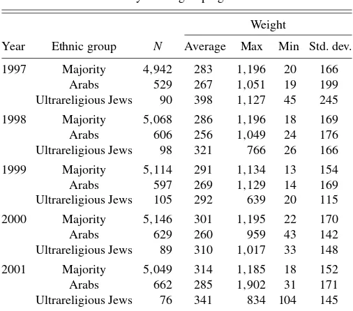
Table 1 provides descriptive statistics of the weights accord-ing to different years and ethnic groupaccord-ings. The population is divided into three groups: two minority groups—Arabs and ul-trareligious Jews (an ulul-trareligious household is defined accord-ing to the school attended by the head of the household), and the rest—referred to as the majority group. The reason for this distinction is that experienced enumerators reported that those groups tend to have different patterns of nonresponse.
In general, one can observe from Table 1 that for all years the average weight of the Arab population is the lowest, mean-ing that they have fewer cases of nonresponse. The maximum weight attached to an observation should be viewed with cau-tion because some of the programs assigning the weights may restrict the weight to be not greater than a certain value. It is worth noting that although the order of average weights ac-cording to the groups remains the same over the years (except
Table 1. Descriptive statistics of household weights by ethnic grouping
Weight
Year Ethnic group N Average Max Min Std. dev.
1997 Majority 4,942 283 1,196 20 166
Arabs 529 267 1,051 19 199
Ultrareligious Jews 90 398 1,127 45 245
1998 Majority 5,068 286 1,196 18 169
Arabs 606 256 1,049 24 176
Ultrareligious Jews 98 321 766 26 166
1999 Majority 5,114 291 1,134 13 154
Arabs 597 269 1,129 14 169
Ultrareligious Jews 105 292 639 20 115
2000 Majority 5,146 301 1,195 22 170
Arabs 629 260 959 43 142
Ultrareligious Jews 89 310 1,017 33 148
2001 Majority 5,049 314 1,185 18 152
Arabs 662 285 1,902 31 171
Ultrareligious Jews 76 341 834 104 145
Source: HES 1997–2001, excluding the observations of East Jerusalem in 1997–1999.
for 1999), the order of the standard deviations of the weights changes.
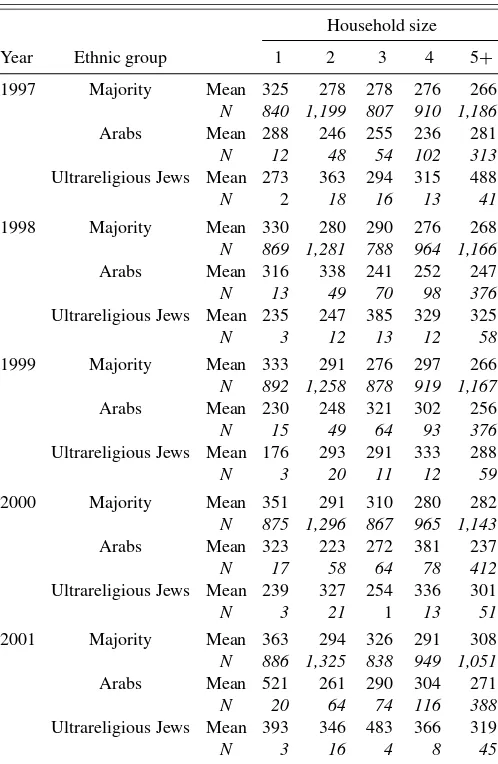
Since the groups differ in household size, which may affect the probability of finding someone at home, Table 2 presents the average weights according to household size. It can be seen that for the majority, household of size 1 has the highest weight, and the rest are similar (year 2001 is different). This may be a result of small households not being at home whereas the elderly, al-though being at home, do not have the patience to complete the questionnaire. (For Arabs, there is no obvious pattern. Nothing can be said about the ultrareligious Jews, since the sample sizes are quite small.)
To summarize: the dependent variable is the weight assigned to each observation by a calibration procedure, intended to rep-resent the entire population. The sample is a stratified sample, but the probability of each dwelling and each person living in a dwelling to be included in the sample is equal. Hence, if the propensity not to be included in the sample is equal, because of either nonresponse or errors on behalf of the agency, the ex-pected weight assigned to each observation should be equal. It may differ between years, if the ratio of sample size to popu-lation changes between years. The weight is treated as an indi-cator of nonresponse. Having described the dependent variable, we now move to describe the results concerning the regression coefficients.
6. EMPIRICAL RESULTS
We turn first to simple regression coefficients. These simple regression coefficients are used in finance (Gregory-Allen and Shalit 1999; Shalit and Yitzhaki 2002), whereas a variation of them has been used for almost 20 years in analyzing the income elasticity of consumption goods (see the survey in Wodon and Yitzhaki 2002). We have estimated the regression coefficients for the years 1997–2001. Since they present a stable picture, only the results for the year 2001 are presented here.
Table 2. Means of household weights by ethnic grouping and household size
Household size
Year Ethnic group 1 2 3 4 5+
1997 Majority Mean 325 278 278 276 266
N 840 1,199 807 910 1,186
Arabs Mean 288 246 255 236 281
N 12 48 54 102 313
Ultrareligious Jews Mean 273 363 294 315 488
N 2 18 16 13 41
1998 Majority Mean 330 280 290 276 268
N 869 1,281 788 964 1,166
Arabs Mean 316 338 241 252 247
N 13 49 70 98 376
Ultrareligious Jews Mean 235 247 385 329 325
N 3 12 13 12 58
1999 Majority Mean 333 291 276 297 266
N 892 1,258 878 919 1,167
Arabs Mean 230 248 321 302 256
N 15 49 64 93 376
Ultrareligious Jews Mean 176 293 291 333 288
N 3 20 11 12 59
2000 Majority Mean 351 291 310 280 282
N 875 1,296 867 965 1,143
Arabs Mean 323 223 272 381 237
N 17 58 64 78 412
Ultrareligious Jews Mean 239 327 254 336 301
N 3 21 1 13 51
2001 Majority Mean 363 294 326 291 308
N 886 1,325 838 949 1,051
Arabs Mean 521 261 290 304 271
N 20 64 74 116 388
Ultrareligious Jews Mean 393 346 483 366 319
N 3 16 4 8 45
Source: HES 1997–2001, excluding the observations of East Jerusalem in 1997–1999.
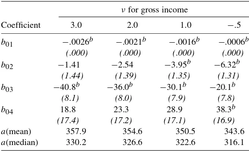
Table 3 presents the regression coefficients of weight on household income, for different values ofν. The higher the pa-rameterνis, the more the regression stresses the slopes of the regression curve at the lower end of the income distribution. (It is worth noting that the weights given to adjacent slopes are solely determined by the distribution of the independent variable andν. They should not be confused with the depen-dent variable of the regression, which is the weight assigned to an observation.) As can be seen, the regression coefficients are negative, which means that the higher the income is, the
Table 3. Regression coefficients of household weight on gross income per household, by extended Gini parameter (ν)
νfor gross income
Coefficient 3 2 1 −.5
b −.0025∗ −.0022∗ −.0017∗ −.0007∗
SE(b) .0003 .0003 .0002 .0001
a(mean) 348.3 342.8 335.7 321.0
a(median) 320.7 314.9 307.8 293.2
Source: HES 2001. Units of income—New Israeli Shekel per month.
∗Indicates a value significantly different than 0 (atα=.05).
lower is the weight assigned to observations, implying that non-response declines with income. For example, a value of−.0022 (obtained forν=2) means that a unit increase in income will decrease the dependent variable (weight) by .0022. The average weight is the ratio of the sample size to the population. There-fore, the value of (−.0022) divided by the average weight gives the percentage rate of the increase in response rate with a unit increase in income. Even when high-income groups are stressed (ν= −.5), we still have a significant negative regression co-efficient. The interpretation of this finding is that we have a monotonic relationship between nonresponse and income. We have checked the pattern for the years 1997–2000 and found the same pattern. To save space the results are not presented.
The rest of Table 3 presents the two versions of the constant term. One presents the constant term when the regression line passes through the median and the other when it passes through the mean. It is interesting to note that the difference between the two is around 28 witha(mean)higher thana(median). This is an indication that the error term tends to be asymmetric. It is not clear to us whether this kind of result, that is, that the difference in the constant terms is independent of the slopes, is a coincidence or is a property of the extended Gini regression procedure.
Table 4 presents the simple regression coefficients of weight on household size. As in the regression on income, the larger the family size, the higher the value of the regression coefficient (in absolute value), and in all cases, the signs of the regression coefficients are negative. This means that nonresponse is higher among small households. Note that as before, the constant term of the regression passing through the mean is larger than the constant term of the regression passing through the median, but again, the difference between the two constants is around 28.
It is interesting that although the differences in the regres-sion coefficients are relatively large, the differences in the stan-dard errors are relatively small. Further research and additional results from different datasets are needed to form an opinion regarding this issue.
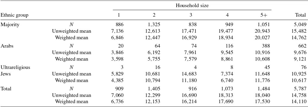
Tables 5a and 5b present the multiple regression coefficients with gross income, household size, and dummy variables for being a member of a minority group (Arabs, ultrareligious Jews) as the independent variables. In Table 5a, the Gini re-gression method is used with a choice of values forν, whereas in Table 5b the OLS method is used for the entire sample and then for each quartile (by income) separately.
Table 4. Regression coefficients of household weight on household size, by extended Gini parameter (ν)
νfor household size
Coefficient 3.0 2.0 1.0 −.5
b −12.2∗ −10.6∗ −8.5∗ −3.5∗
SE(b) 1.4 1.3 1.1 1.2
a(mean) 354.1 347.5 339.3 321.4
a(median) 326.7 320.0 311.1 293.2
Source: HES 2001.
∗Indicates a value significantly different than 0 (atα=.05).