Manajemen | Fakultas Ekonomi Universitas Maritim Raja Ali Haji 073500102288618702

(1)

Full Terms & Conditions of access and use can be found at

http://www.tandfonline.com/action/journalInformation?journalCode=ubes20

Download by: [Universitas Maritim Raja Ali Haji] Date: 13 January 2016, At: 00:38

Journal of Business & Economic Statistics

ISSN: 0735-0015 (Print) 1537-2707 (Online) Journal homepage: http://www.tandfonline.com/loi/ubes20

Was There a Riverside Miracle? A Hierarchical

Framework for Evaluating Programs With Grouped

Data

Rajeev H Dehejia

To cite this article: Rajeev H Dehejia (2003) Was There a Riverside Miracle? A Hierarchical Framework for Evaluating Programs With Grouped Data, Journal of Business & Economic Statistics, 21:1, 1-11, DOI: 10.1198/073500102288618702

To link to this article: http://dx.doi.org/10.1198/073500102288618702

Published online: 01 Jan 2012.

Submit your article to this journal

Article views: 40

(2)

Was There a Riverside Miracle? A Hierarchical

Framework for Evaluating Programs With

Grouped Data

Rajeev H.

Dehejia

Department of Economics and SIPA, Columbia University, New York, NY 10027 (rd247@columbia.edu) National Bureau of Economic Research, Cambridge, MA 02138

This article discusses the evaluation of programs implemented at multiple sites. Two frequently used methods are pooling the data or using xed effects (an extreme version of which estimates separate models for each site). The former approach ignores site effects. The latter incorporates site effects but lacks a framework for predicting the impact of subsequent implementations of the program (e.g., would a new implementation resemble Riverside?). I present a hierarchical model that lies between these two extremes. Using data from the Greater Avenues for Independence demonstration, I demonstrate that the model captures much of the site-to-site variation of the treatment effects but has less uncertainty than estimating the treatment effect separately for each site. I also show that when predictive uncertainty is ignored, the treatment impact for the Riverside sites is signicant, but when predictive uncertainty is considered, the impact for these sites is insignicant. Finally, I demonstrate that the model extrapolates site effects with reasonable accuracy when the site being predicted does not differ substantially from the sites already observed. For example, the San Diego treatment effects could have been predicted based on their site characteristics, but the Riverside effects are consistently underpredicted.

KEY WORDS: Bayesian methods; Predictive uncertainty; Site effects.

1. INTRODUCTION

This article discusses the problem of evaluating and predict-ing the treatment impact of a program that is implemented at multiple sites; at a methodological level, it illustrates the use of hierarchical models for data that have a group (e.g., site) structure. Many programs operate or are evaluated at mul-tiple sites, including the National Supported Work Demon-stration, Job Training Partnership Act (JTPA) DemonDemon-stration, and Greater Avenues for Independence (GAIN). This article presents a framework for dealing with multisite programs and (using data from GAIN) argues that the site structure of data must be considered when evaluating a program.

When data have a site structure, there is a distinction between evaluating a program and predicting the outcome in subsequent implementations. Evaluation is a historical ques-tion; one wants to determine what the impact of a program was in a particular site at a particular point in time. In con-trast, prediction relates to future implementations of a pro-gram, either at one or more of the sites where the evaluation was conducted or possibly at a new site. Both kinds of ques-tions are potentially challenging with multisite programs.

The challenge with evaluation is how and to what extent data should be pooled across sites. Differences across sites can emerge for two reasons. There can be differences in the composition of participants, which is addressed relatively eas-ily if a sufcient number of the participants’ characteristics are observed. But there can also be site-specic variation in treatment, with differences ranging from the services offered to administrative philosophy. To the extent that site-specic effects are absent and that one can condition on individual characteristics, the benet of pooling the data is increased pre-cision in the estimates. This can be particularly important if there are very few observations at some sites. If site effects are present, the data can still be pooled if one allows for xed

effects. However, this leads to difculties in predicting the impact of the program.

Using xed effects or, more generally, estimating separate models for each site limits one to thinking of subsequent implementations of the program as being identical to one of the original sites, because there is no framework to account for predictive uncertainty regarding the value of the xed-effects or site-specic model. This is true both when predict-ing the impact at one of the sites in the evaluation (in which case one wants to redraw for the site effect) and when pre-dicting the impact at a new site.

The solution that this article proposes is hierarchical mod-eling (see Gelman, Carlin, Stern, and Rubin 1996 and also Rossi, McCulloch, and Allenby 1995; Chamberlain and Imbens 1996; Geweke and Keane 1996 for other applications of these methods). Hierarchical modeling is a middle ground between xed-effects modeling and pooling the data without xed effects. Hierarchical modeling is somewhat familiar in the literature through the related concept of meta-modeling (see Cooper and Hedges 1994). Meta-modeling involves link-ing the outcomes of separate studies on the same topic through an overarching model. It can also be used to model site effects; for example, Card and Krueger (1992) estimated cohort– and state-of-birth–specic returns to schooling and then use a meta-model to relate these to measures of school quality. The method adopted in this article is a Bayesian version of meta-modeling.

The model has three layers. The rst layer involves separate models for each site, the second layer links the coefcients

©2003 American Statistical Association Journal of Business & Economic Statistics January 2003, Vol. 21, No. 1 DOI 10.1198/073500102288618702 1

(3)

2 Journal of Business & Economic Statistics, January 2003

of the site models through a regression-type meta-model, and the third layer consists of prior distributions for the unknown parameters. Thus a hierarchical model combines features of the xed-effects and pooled models but also allows for inter-mediate models. Compared to standard xed- (or random-) effects model, it allows for site-specic estimation of all coef-cients, not just the constants. Furthermore, participants across sites are not assumed to be exchangeable conditional on indi-vidual characteristics, but rather to be exchangeable within sites conditional on individual characteristics. Finally, a prior distribution is used to model the extent to which site effects are believed to be drawn from a common distribution—namely, the extent to which coefcients should be “smoothed” across sites, or observations from one site should inuence estimates in other sites.

This approach is applied to data from the GAIN demon-stration, a labor-training program implemented in 6 California counties at 24 sites (see Riccio, Friedlander, and Freedman 1996). For the GAIN data, the primary benet of applying hierarchical models is in terms of prediction rather than evalu-ation. Each site has a sufcient number of observations so that the gain in precision from pooling data from other sites is lim-ited. However, the predictive questions are of central impor-tance. Much attention in the GAIN program focused on the Riverside county implementation, which was viewed as being highly successful and distinct from other counties (see, e.g., Nelson 1997).

The interest here lies in discovering the extent to which a hierarchical model succeeds in capturing these site effects that have been viewed as being primarily qualitative in nature. I focus on three issues. First, do data from other sites help in evaluating the program at a given site? Second, if one imag-ines reimplementing a GAIN-type program, would one be able to predict the site effects based on the observable characteris-tics of each site, and how important is predictive uncertainty? Third, how well can the model extrapolate to sites that have not been observed?

Other work on multisite evaluation issues includes that of Heckman and Smith (1996), Hotz, Imbens, and Mortimer (1998), and Hotz, Imbens, and Klerman (2000). Heckman and Smith (1996) analyze the sensitivity of experimental estimates to the choice of sites used in the analysis and to different meth-ods of weighting the pooled data. They establish that there is signicant cross-site variation in the data from the JTPA evalu-ation. Hotz et al. (1998) analyze the importance of site effects in the Work Incentives demonstration using the key insight that even if there is heterogeneity in the treatment available at each site, control groups excluded from the treatment still should be comparable. They nd that control group earnings are comparable across sites when controlling both for individ-ual characteristics and for site-level characteristics; however, posttreatment earnings for the treated group are not compara-ble, suggesting the existence of heterogeneity in the treatment. Taken together, these works motivate the use of a hierarchi-cal model, which explicitly allows for site effects in treatment and control earnings and directly incorporates site-level char-acteristics.

The work of Hotz et al. (2000) is complementary to this article. It examines the GAIN data using the same framework

used by Hotz et al. (1998), and the ndings are also simi-lar. The authors are able to adjust for differences in control group earnings using individual and site-level characteristics. However, differences remain in posttreatment earnings. The authors thus present a series of differences-in-differences esti-mates that, inter alia, suggest that the treatment available at Riverside did have a positive effect relative to the treatment offered at other sites. This nding is discussed in Section 5.

This article is organized as follows. Section 2 describes the GAIN program, and Section 3 discusses key features of the GAIN data. Section 4 outlines the hierarchical model. Section 5 presents the results, and Section 6 concludes.

2. THE GREATER AVENUES FOR INDEPENDENCE PROGRAM

The GAIN program began operating in California in 1986, with the aim of “increasing employment and fostering self-sufciency” among AFDC recipients (see Riccio et al. 1994). In 1988, six counties—Alameda, Butte, Los Angeles, River-side, San Diego, and Tulare—were chosen for an experimen-tal evaluation of the benets of GAIN. A subset of Aid to Families With Dependent Children (AFDC) recipients (single parents with children age 6 or older and unemployed heads of two-parent households) were required to participate in the GAIN experiment.

Potential participants from the mandatory group were referred to a GAIN orientation session when they visited an Income Maintenance ofce either to sign up for welfare or to qualify for continued benets. As a result, the chronology of the data and subsequent results are in experimental time, rather than calendar time. No sanctions were used if individ-uals failed to attend the orientation sessions. However, once individuals started in the GAIN program, sanctions were used to ensure their ongoing participation. At the time of enroll-ment into the program, various background characteristics were recorded for both treatment and control units, including demographic characteristics, results of a reading and mathe-matics prociency test, and data on 10 quarters of pretreatment earnings, AFDC participation, and food stamp receipts.

Of those who attended the orientation session, a fraction was randomly assigned to the GAIN program, and the oth-ers were prohibited from participating in GAIN (but could of course participate in non-GAIN employment-creating activi-ties). Each of the counties randomized a different proportion of its participants into treatment, ranging from a 50–50 split in Alameda to an 85–15 split in San Diego (see Table 1). Because assignment to treatment was random, the distribution

Table 1. The Sample

Los San Alameda Butte Angeles Riverside Diego Tulare

GAIN:

Treated group 685 1717 3730 5808 8711 2693 Control group 682 458 2124 1706 1810 1146

Total 1367 2175 5854 7514 10521 3839

Number of sites 1 1 5 4 8 5

NOTE: The GAIN sample sizes are from the public use ’le of the GAIN data.

(4)

Dehejia: Evaluating Programs With Grouped Data 3

of pretreatment covariates is balanced across the treatment and control groups. In terms of the chronology of data gathering, “experimental” time (which I also call “posttreatment” time) begins when individuals attend the GAIN orientation session. Thus the early stages of experimental time coincide with the education and training of GAIN participants.

In the GAIN experiment, the treatment is participating in the GAIN program and the control is receiving standard AFDC benets. The GAIN program works as follows: Based on test results and an interview with a case manager, participants were assigned to one of two activities. Those deemed not to be in need of basic education are referred to a job search activity (which lasts about 3 weeks); those who did not nd work are placed in job training (which includes vocational or on-the-job training and paid or unpaid work experience, lasting about 3–4 months). Those deemed to be in need of basic edu-cation can choose to enter the job search immediately, but if they fail to nd a job, then they are required to register for preparation for a General Educational Development certicate, Adult Basic Education, or English as a Second Language pro-grams (lasting 3–4 months). Participants are exempted from the requirement to participate in GAIN activities if they nd work on their own.

The counties in the GAIN experiment varied along two important dimensions. First, the composition of program par-ticipants varied, because counties chose to focus on particular subsets of their welfare populations, and the populations dif-fered. For example, Alameda and Los Angeles Counties con-ned themselves to the subset of long-term welfare recipients (i.e., individuals who already received welfare for 2 years or longer). The second difference is that the subtreatment offered within each county varied because of differences in adminis-trative philosophy. The approach followed by Riverside, which has received much attention, was to focus on job rather than skills acquisition. Both are part of the program, but River-side’s emphasis was on the former. In contrast, counties like Alameda focused more on skill acquisition. The model allows for differences in composition by conditioning on pretreat-ment covariates and differences in the treatpretreat-ment by allowing for site effects.

3. THE GREATER AVENUES FOR INDEPENDENCE DATA

Table 2 presents the 6 counties that participated in the GAIN experiment, broken down in terms of their 24 admin-istrative sites. The counties vary from one-site counties, such as Alameda, to multisite counties, such as Los Angeles and San Diego. This article analyzes the results at the site level, because with six counties there is minimal scope for model-ing site effects. Table 2 also presents the background char-acteristics of each site. Note that the average number of children varies from more than four in site 21 to slightly more than two in site 6. The proportion of Hispanics in the sample varies from a low of 0 in site 13 to more than 50% in sites 14 and 24.

Table 2 also shows signicant variation in the treatment impact across sites. The second-to-the-last row lists the aver-age quarterly treatment effect. The treatment impact ranges

from a high of $212 for site 5 (in Riverside) to a low ofƒ$133

for site 17 (in Tulare). In the last row, the treatment effect is estimated conditioning on pretreatment covariates through an OLS regression. The estimates are similar, ranging from

ƒ$90 to $292. The sites consistently showing the highest and

most signicant impacts are those from Riverside (sites 2–5). Their treatment impacts range from $149 to $292 and are sig-nicantly different from 0. The worst performing county is Tulare, for which some of the impacts are negative and all of the impacts are statistically insignicant.

4. THE ECONOMETRIC MODEL

An important feature of the data that inuences the mod-eling strategy is the large proportion of 0s in the outcome earnings. With as many as 75% of the outcomes being 0, the model must explicitly account for the mass point in the earn-ings distribution. The most parsimonious model for dealing with a mass point at 0 is the Tobit model.

4.1 The Hierarchical Model

The hierarchical model (see Gelman et al. 1996) is a gener-alization of the regression model that allows each site to have its own value for the coefcients,

Yü

whereYijtis observed income andYijtü is a latent variable such

that Y_ijt D0 if Yü citj71 Tiis a treatment indicator (1 if treated, 0 otherwise), and

citj is a vector of exogenous pretreatment variables.

Let ‚0

jD4‚j1¢ ¢ ¢‚jM5, where mD11 : : : 1 M indexes the

regressors. The model assumes a constant variance across

sites. The key feature of the model is that the‚’s are linked

through a further model,

where zj are a set of site characteristics used to model the

site coefcients. The model for‚serves as a prior distribution

with respect to the base model for earnings.

The model is completed by dening priors for the parame-ters,

The values for r 1 Q1 d, and D are chosen to correspond to a

noninformative prior. The prior onèƒ1 _{determines the degree}

of smoothing that the model performs. The estimate of the ‚’s for each site are a precision-weighted average of the OLS

estimates within each site and the‚’s predicted by the model

in (2) (see the Appendix). The weight in turn is inuenced by

the prior for èƒ1_{. The Wishart prior can be interpreted as}

previous observations with variance Kƒ1_{. When} _Kƒ1 _reects

(5)

4

Jo

urn

al

of

Busi

ness

&

Eco

nomi

c

S

tati

sti

cs

,

January

2

003

Table 2. Site Characteristics From the GAIN Experiment

Butte Riverside San Diego Tulare Alameda Los Angeles

Site 1 Site 2 Site 3 Site 4 Site 5 Site 6 Site 7 Site 8 Site 9 Site 10 Site 11 Site 12 Site 13 Site 14 Site 15 Site 16 Site 17 Site 18 Site 19 Site 20 Site 21 Site 22 Site 23 Site 24 Variable (2165) (3364) (2052) (1358) (706) (755) (1457) (1104) (678) (1853) (2111) (1897) (630) (500) (531) (1060) (864) (880) (1360) (835) (842) (1485) (1888) (800)

Number of children

Mean 2.5 2.69 2.84 2.84 2.6 2.2 2.79 2.5 2.36 2.35 2.6 2.35 4.02 2.91 3.12 3.05 3 3.04 2.38 3.5 4.3 3.23 3.84 3.77 (SE) (1.74) (1.85) (1.88) (2.04) (1.64) (1.56) (1.91) (1.67) (1.5) (1.65) (1.78) (1.54) (2.48) (1.86) (2.1) (2.03) (2) (1.86) (1.57) (2.2) (2.55) (2.19) (2.27) (2.31) Reading test score

Mean 238.37 232.94 232.56 230 233.18 237.56 230.6 237.94 236.38 234.28 231.05 237.59 198.55 230.69 231.29 231.96 231.21 232.82 199.8 230.01 224.32 225.62 225.29 224.92 (SE) (13.14) (14.42) (18.11) (15.18) (12.17) (14.9) (15.82) (15.06) (14.26) (15.34) (20.24) (14.18) (38.69) (14.44) (15.29) (13.72) (14.06) (13.65) (77.95) (18.22) (16.44) (13.59) (14.72) (16.17) Grade

Mean 10.96 10.78 10.66 9.59 10.98 11.79 10.53 11.41 11.54 11.39 10.38 11.31 6.55 9.6 9.38 9.44 10.17 9.87 10.79 9.43 7.65 9.41 9.62 7.54 (SE) (2.61) (2.56) (2.64) (3.24) (1.95) (2.46) (2.89) (2.2) (2.17) (2.37) (3.05) (2.04) (4.23) (3.18) (3.42) (3.26) (2.75) (3.5) (3.03) (3.47) (3.85) (3.74) (3.56) (3.91) Previous training experience

Mean .22 .23 .27 .14 .22 .1 .12 .04 .04 .08 .11 .14 .12 .07 .24 .24 .24 .12 .24 .18 .12 .05 .16 .17 (SE) (.42) (.42) (.45) (.35) (.42) (.3) (.32) (.2) (.18) (.28) (.31) (.34) (.33) (.25) (.43) (.43) (.43) (.32) (.43) (.38) (.32) (.22) (.37) (.37) Hispanic

Mean .07 .24 .19 .57 .18 .14 .3 .17 .19 .17 .55 .1 0 .62 .45 .32 .39 .36 .08 .36 .27 .2 .16 .76 (SE) (.25) (.43) (.39) (.5) (.38) (.34) (.46) (.37) (.39) (.38) (.5) (.3) (0) (.48) (.5) (.47) (.49) (.48) (.27) (.48) (.44) (.4) (.36) (.43) Black

Mean .03 .18 .09 .09 .19 .11 .51 .08 .27 .33 .12 .07 0 .01 0 .01 .11 .02 .64 .12 .08 .45 .61 .06 (SE) (.17) (.38) 387 (.28) (.39) (.32) (.5) (.27) (.44) (.47) (.33) (.26) (.06) (.09) (.06) (.09) (.31) (.14) (.48) (.32) (.28) (.5) (.49) (.23) Lagged earnings, 1 quarter before treatment

Mean 451 387 335 493 343 481 352 540 524 443 499 509 286 490 512 439 464 522 142 145 186 174 158 87 (SE) (1034) (1074) (1007) (1136) (1061) (1115) (846) (1220) (1174) (1118) (1189) (1111) (531) (1022) (1085) (987) (1009) (1360) (606) (477) (443) (604) (616) (444) Average quarterly treatment impact

Treatment effect 179 141 197 161 212 194 ƒ41 40 179 141 197 161 212 194 ƒ41 40 ƒ133 ƒ12 76 80 87 ƒ10 10 ƒ59 (SE) (57) (42) (55) (66) (82) (117) (70) (94) (112) (72) (71) (70) (84) (96) (87) (61) (75) (79) (46) (52) (40) (43) (36) (46) Average quarterly treatment impact, conditional on covariates

Treatment effect 145 149 149 190 292 213 21 49 116 195 39 104 ƒ90 ƒ15 25 80 ƒ18 ƒ2 84 108 80 ƒ6 ƒ7 ƒ50 (SE) (50) (39) (39) (56) (72) (109) (64) (90) (104) (65) (62) (65) (77) (87) (77) (53) (68) (62) (41) (49) (37) (39) (32) (44)

NOTE: For each site, the sample size is given in parentheses.

(6)

high variance, this will pull up the estimate ofè (and hence

reduce the estimated prior precision,èƒ1_{) and lead to a lower}

weight being placed on the common prior for the‚’s and a

higher weight placed on the ‚_j’s estimated within each site

(hence minimal smoothing). The values used for this prior range from minimal smoothing to maximal smoothing. Esti-mation is undertaken using a Gibbs sampler (outlined in the Appendix).

The hierarchical model could also be estimated using max-imum likelihood methods, but the limitation of doing this is that the number of sites is very small. This not only ren-ders standard asymptotic approximations of the distributions of parameters unreliable, but also makes it hard to estimate

parameters such as èƒ1 _{exclusively from the data without}

using a prior.

4.2 The Predictive Distribution

Because the object of interest for the policy question is earnings and only indirectly the parameters, I generate the pre-dictive distribution, the distribution in the space of outcomes that captures all of the uncertainty (both intrinsic uncertainty and parameter uncertainty) from the model. This distribution is simulated by repeatedly drawing for parameter values from their posterior distribution and then drawing from the outcome distribution conditional on observed data and parameters.

5. THE RESULTS

Here the model outlined in Section 4 is implemented on the GAIN data, using age, education, number and age of chil-dren, previous participation in a training program, reading and writing test scores, ethnicity, and pretreatment earnings as pretreatment individual characteristics. These are interacted with the treatment indicator, so that the model allows for the site effect for treatment and control earnings to be different. The mean characteristics of participants (including the mean number of children, mean reading score, mean level of edu-cation, mean age, and mean pretreatment earnings) are used as the site characteristics. The Gibbs sampler outlined in the Appendix produces estimates of the posterior distribution of the parameters. These are then used to produce a predictive distribution of earnings (under treatment and control) for each individual. The predictive distributions are then averaged over the individuals at a site to produce an estimate of the site impact.

5.1 Site Effects and Evaluation

This section examines to what extent observations from other sites help evaluate the program at a particular site. In general, this is an empirical question, and the answer depends on the dataset under consideration. From Section 4, recall that the degree of smoothing performed by the hierarchical model

depends onèƒ1_{, and the estimate of this parameter is in turn}

inuenced byKƒ1_{, which is a prior. If}_Kƒ1_{is small, then this}

pulls down the estimate ofèƒ1_{, which in turn means that a}

lower weight is put on the common prior and a higher weight

is put on the within-site estimates. By varyingKƒ1_{, the results}

of the hierarchical model range from fully pooled to site-by-site estimates. Because the number of site-by-site observations typi-cally is small (24 for the GAIN data), the prior will have a

substantial inuence on the nal estimate ofèƒ1_{. The}

empir-ical question then becomes to what extent does the choice of smoothing prior inuence the estimate of earnings and the treatment effect within each site.

Table 3 presents estimates of the Tobit model under a range of assumptions. In row (1), the earnings are estimated using a nonhierarchical Tobit, estimated from the pooled data; these estimates ignore site effects. In row (2) Tobits are estimated individually for each site. The next two rows present estimates from the hierarchical Tobit model. In row (3) the prior is cho-sen so that minimal smoothing is performed, and in row (4) the prior is chosen to induce a greater degree of smoothing. Of the four models, the site-by-site Tobit and the minimally smoothed hierarchical models should be nearly identical; when the prior is selected for minimal smoothing, it essentially induces site-by-site Tobits. This is conrmed by comparing rows (2) and (3).

The pooled estimates and those from the site-by-site (or minimally smoothed) models differ substantially, although not dramatically. For treatment (control) earnings, the mean

dif-ference is $25 (ƒ$6), with a mean absolute deviation of $69

($56). This reects the obvious fact that the site-by-site mates bounce around more than the pooled estimates. The esti-mated treatment effects implied by these models are depicted in Figure 1 (along with the 2.5 and 97.5 percentiles of the predictive distributions of the average treatment effect). The by-site estimates represent unbiased estimates of the site-treatment effects. The advantage of pooling is reected in the lower standard errors of the estimates in Figure 1(a).

Figure 1(c) depicts the estimated treatment effect from the smoothed hierarchical model. As would be expected, the esti-mates lie between those of the other two models. They are less dispersed and have somewhat smaller uncertainty bounds than the site-by-site estimates. The mean absolute deviation for the treatment effect with the pooled model is $53, and the 2.5–97.5 percentile uncertainty bounds are narrower by about $17 on average.

Overall, Figure 1 depicts a broadly similar prole of treat-ment effects, but the differences in the uncertainty bounds qualitatively affect the results. In Figure 1(b), 10 of the 24 treatment effects are insignicant (in the sense that the 2.5–97.5 percentile bounds include 0), but only 1 treatment effect with the pooled estimates is insignicant and only 3 treatment effects for the smoothed estimates are insignicant. It is important to note that there is neither an a priori nor an empirical basis to choose between these estimates. If one were forced to pick a single estimate, then the choice would depend on the smoothing prior that could be comfortably adopted. Of course, looking at the range of estimates is also quite informative.

A concrete illustration of the role that site effects can play is given in Table 3, row (5). The counterfactual exercise pre-sented is to assign the individuals from a given site (site 19, Alameda) into the other sites. The same site effects are used as in Table 3, row (3). The thought experiment is to deter-mine earnings for Alameda participants if, for example, they

(7)

6

Jo

urn

al

of

Busi

ness

&

Eco

nomi

c

S

tati

sti

cs

,

January

2

003

Table 3. Average Earnings per Person per Quarter

Butte Riverside San Diego

Model Site 1 Site 2 Site 3 Site 4 Site 5 Site 6 Site 7 Site 8 Site 9 Site 10 Site 11 Site 12

(1) Pooled Treated 614 562 535 564 567 649 535 652 644 599 586 641

(601, 628) (552, 572) (522, 548) (548, 580) (547, 586) (629, 670) (519, 550) (635, 672) (623, 667) (585, 613) (572, 600) (625, 655)

Control 499 446 422 464 447 518 424 527 517 475 474 516

(485, 512) (436, 457) (410, 434) (449, 479) (428, 467) (498, 539) (410, 436) (509, 543) (497, 537) (463, 488) (461, 486) (502, 530)

(2) Separate Treated 533 604 596 672 566 728 480 613 664 594 561 553

(512, 555) (587, 622) (573, 619) (644, 702) (525, 608) (683, 772) (456, 505) (581, 648) (619, 708) (570, 620) (537, 582) (531, 579)

Control 407 421 366 483 343 559 440 563 557 467 506 465

(384, 431) (403, 441) (344, 388) (452, 515) (302, 384) (499, 620) (409, 470) (521, 605) (500, 616) (438, 501) (478, 537) (434, 496) (3) Hierarchical, Treated 533 605 595 672 563 726 481 611 666 596 562 554

no smoothing (513, 555) (586, 623) (570, 620) (644, 703) (525, 605) (684, 772) (455, 507) (579, 644) (622, 712) (573, 618) (540, 586) (531, 578)

Control 407 422 365 485 342 558 442 560 558 466 507 465

smoothed (571, 609) (531, 555) (510, 539) (552, 590) (535, 578) (597, 650) (480, 512) (658, 712) (614, 667) (544, 576) (561, 592) (608, 640)

Control 436 417 409 500 420 470 385 544 502 413 486 479

(418, 456) (405, 429) (395, 423) (479, 520) (400, 441) (444, 494) (368, 402) (516, 570) (474, 530) (397, 430) (469, 504) (462, 498)

(5) Alameda Treated 401 525 545 538 483 536 418 494 527 472 479 472

participants (383, 418) (505, 544) (524, 567) (514, 561) (449, 515) (508, 562) (400, 436) (472, 518) (499, 557) (454, 492) (463, 496) (453, 492)

in other sites Control 335 354 306 333 263 365 371 435 357 323 416 403

predicting (365, 1289) (321, 1282) (276, 1251) (347, 1305) (282, 1229) (384, 1383) (293, 1187) (369, 1382) (404, 1471) (311, 1474) (333, 1366) (348, 1367)

effects site Control 444 400 387 495 392 451 386 514 475 392 457 453

(221, 1371) (204, 1376) (187, 1203) (254, 1358) (193, 1219) (187, 1511) (202, 1255) (227, 1375) (225, 1547) (186, 1477) (221, 1499) (217, 1550)

(7) Predicting Treated 609 502 477 537 497 622 489 710 645 542 545 624

site effects, (311, 2302) (293, 2015) (283, 2045) (330, 2016) (234, 1872) (303, 3070) (276, 2557) (377, 2611) (276, 2389) (289, 2594) (277, 2307) (297, 2131)

dropping Control 458 397 390 501 402 431 379 503 459 385 447 451

observations (215, 3262) (185, 2442) (195, 2598) (251, 2857) (176, 2611) (140, 2783) (168, 2607) (174, 3503) (183, 2431) (159, 3055) (213, 2964) (167, 2014) from that site

site effects, (343, 1936) (2, 7408) (0, 7422) (1, 7693) (1, 6646) (4, 6799) (3, 6407) (9, 6752) (8, 6835) (7, 7088) (2, 6570) (6, 6524)

observations (238, 2142) (6, 3570) (6, 3793) (6, 3895) (11, 3616) (11, 2991) (13, 3123) (33, 3261) (22, 2819) (29, 3019) (20, 3209) (16, 2619) from that county

(continued)

(8)

Dehejia:

Eval

uating

Program

s

W

ith

G

rouped

Data

7

Table 3 (continued)

San Diego Tulare Alameda Los Angeles

Model Site 13 Site 14 Site 15 Site 16 Site 17 Site 18 Site 19 Site 20 Site 21 Site 22 Site 23 Site 24

(1) Pooled Treated 410 601 581 560 600 581 453 401 387 413 403 307

(390, 428) (577, 625) (556, 607) (542, 575) (582, 622) (561, 601) (439, 466) (384, 418) (371, 402) (401, 426) (392, 415) (294, 323)

Control 344 504 480 460 491 469 337 297 299 309 296 223

(327, 362) (480, 527) (458, 503) (445, 477) (472, 510) (450, 487) (326, 350) (283, 311) (286, 314) (298, 321) (286, 305) (211, 236)

(2) Separate Treated 561 620 585 488 510 516 282 323 427 289 303 175

(520, 601) (570, 668) (545, 629) (456, 522) (476, 542) (483, 547) (259, 303) (294, 350) (394, 460) (269, 307) (286, 321) (156, 195)

Control 620 637 534 423 530 509 227 251 324 285 286 200

no smoothing (522, 602) (564, 666) (540, 632) (460, 520) (480, 548) (485, 552) (262, 300) (293, 349) (394, 460) (268, 308) (284, 322) (154, 197)

Control 617 630 537 423 530 513 226 251 323 286 288 200

Smoothed (489, 563) (606, 674) (593, 648) (533, 576) (576, 620) (563, 605) (322, 364) (284, 321) (393, 444) (310, 339) (322, 357) (179, 212)

Control 547 538 561 488 524 506 268 254 384 274 278 198

(499, 592) (500, 576) (530, 590) (465, 510) (497, 548) (488, 525) (251, 286) (236, 271) (358, 411) (260, 289) (263, 295) (180, 217)

(5) Alameda Treated 487 445 398 403 361 387 281 367 455 274 361 267

participants (453, 522) (412, 480) (368, 431) (377, 431) (336, 385) (361, 411) (260, 301) (337, 399) (419, 497) (257, 294) (341, 384) (239, 296)

in other sites Control 749 439 403 316 383 370 226 282 282 315 332 275

predicting (263, 1474) (452, 1306) (374, 1111) (325, 1072) (362, 1138) (376, 1224) (191, 725) (175, 779) (290, 1134) (189, 805) (188, 858) (96, 483)

effects site Control 641 604 548 480 514 481 286 241 397 246 257 184

(326, 2082) (348, 1613) (318, 1615) (270, 1416) (313, 1498) (278, 1562) (143, 991) (140, 1011) (188, 1716) (152, 972) (138, 1045) (90, 1020)

site effects, (191, 4007 (407, 2786) (368, 2141) (291, 2531) (307, 1983) (338, 1987) (174, 5522) (149, 1834) (276, 3258) (175, 1582) (150, 3694) (93, 3049)

observations (180, 8996) (223, 3964) (260, 2964) (274, 3152) (249, 2663) (268, 2696) (332, 4635) (117, 2948) (271, 5806) (119, 2230) (107, 3402) (71, 4930) from that site

site effects, (5, 5153) (4, 6881) (2, 7844) (2, 7287) (2, 7591) (2, 7942) (178, 879) (5, 9228) (12, 8219) (4, 8013) (1, 8072) (4, 8998)

Observations (76, 3840) (22, 4287) (10, 4250) (12, 4423) (7, 4855) (15, 4442) (132, 881) (40, 3840) (151, 4040) (39, 3050) (26, 4224) (96, 3974) from that

county

NOTE: The table presents the mean and in parentheses the 2.5 and 97.5 percentiles of the predictive distribution of average earnings per person per quarter. In rows 1–4 and rows 6–8, earnings are predicted for the original treatment and control participants at each site, under the speci’ed models. In row 5, earnings are predicted for the Alameda treatment and control participants, if they had been located at the speci’ed site.

(9)

Figure 1. Average Treatment Impact per Person per Quarter. The ’gure depicts the mean and 2.5 and 97.5 percentiles of the predictive distribution of the average treatment effect per person per quarter at each site under the speci’ed models. (a) Corresponds to Table 3, row (1), (b) corresponds to Table 3, row (3), and (c) corresponds to Table 3, row (4).

had entered the program in the environment of Riverside. As the sites are varied, variation is seen in both estimated earn-ings and the treatment impact for these individuals. The level of treatment (control) earnings varies from $267 ($226) in site 24 (site 19) to $545 ($749) in site 3 (site 13). The treatment

effect varies from ƒ$262 in site 13 to $239 in site 3. Note

that the Alameda participants are predicted to have a higher treatment effect if they had participated in the Riverside treat-ment. Hotz et al. (2000) reported similar ndings, but noted that this effect attenuates beyond the 13 quarters of earnings observed in the current dataset.

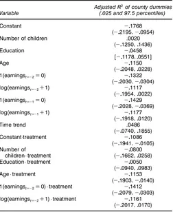
5.2 Are There County Effects?

The GAIN data have both a site structure and a county structure. The model discussed in Section 5.1 ignores the county structure. The difculty in dealing with county-level effects is that only six counties are observed in the dataset. With six observations, it would be difcult to estimate even a single-parameter model. Table 4, however, suggests that county effects are not a source of concern in the GAIN data once site effects have been modeled. It summarizes the explanatory power of county-level dummies on the site-level

estimated coefcients of the model (using adjusted R2_{). The}

2.5 and 97.5 percentile intervals for adjusted R2_{are very broad}

and are less than or include 0.

5.3 Insample Predictive Uncertainty

Thus far the analysis has taken the prole of site effects as given. In this section the GAIN program is examined from a predictive perspective. If the GAIN program were

Table 4. Explanatory Power of County Dummies Conditional on Site Characteristics

Adjusted R2_{of county dummies}

Variable (.025 and 97.5 percentiles)

Constant ƒ01768

(ƒ021951ƒ00954)

Number of children .0020

(ƒ01250101436)

Education ƒ00458

[ƒ01178100551]

Age ƒ01150

(ƒ02048100228)

1(earningstDƒ2D0) ƒ01322

(ƒ020301ƒ00304)

log(earningstDƒ2C1) ƒ01117

(ƒ01954100022)

1(earningstDƒ1D0) ƒ01429

(ƒ020281ƒ00369)

log(earningstDƒ1C1) ƒ01177

(ƒ01918100120)

Time trend .0486

(ƒ00740101855)

Constant¢treatment ƒ01086

(ƒ019411ƒ00105)

Number of ƒ00800

children¢treatment (ƒ01662100258)

Education¢treatment ƒ00050

(ƒ00940100983)

Age_¢treatment ƒ01153

(ƒ019031ƒ00140)

1(earningstDƒ2D0)¢treatment ƒ01412

(ƒ020791ƒ00303)

log(earningstDƒ2C1)¢treatment ƒ01161

(ƒ02017100170)

NOTE: The table presents the mean and in parentheses the 2.5 and 97.5 percentiles of the predictive distribution of the adjusted R2_{of a regression of site coef’cients on county-level}

dummies.

(10)

to be reimplemented, allowing for new site effects in each site (hence predictive uncertainty), then would the treatment effects be signicant? In Table 3, row (6), the parameters for each site are reestimated based on each site’s characteristics. The relevant comparison is to the estimates in Table 3, row (3), which ignore uncertainty in the site effects. The immediate observation is that the results are quite similar, typically within $50. At one level, this may seem trivial; because the data for a given site are included in the estimation, it may not seem surprising that the treatment can be predicted with reasonable accuracy. But the result is not trivial, because for each site new site parameters are drawn based on the hierarchical model and predictions are based on these parameters. So, for example, when the outcome for site 6 is predicted, the characteristics of its participants imply a set of site characteristics, which in turn produce a set of site parameters that lead to the average earnings estimated.

Nonetheless, the range of uncertainty increases substan-tially. In Table 3, row (3), the 2.5–97.5 percentile intervals of the posterior distributions overlap to a large extent for 11 of 24 sites, and in this sense the treatment effects at these sites are not signicant. In Table 3, row (6), the 2.5–97.5 percentile intervals for average earnings overlap for all 24 sites. In partic-ular, for sites 2, 3, 4, and 5 (the Riverside sites), the posterior 95% probability intervals do not overlap in row (3), but they do overlap in row (6). Overall, the comparison of the two sets of estimates suggests that reestimating the site-specic param-eters for each site successfully replicates a prole of outcomes similar to those obtained for each site in isolation. However, uncertainty increases, in some cases signicantly.

5.4 Out-of-Sample Predictive Uncertainty

An important question regarding site effects is whether the outcomes at a site could be predicted if that site had not been observed in the data. In other words, are site effects so impor-tant that it is difcult or impossible to predict the treatment effect at a given site using data from other sites? To explore this issue, the estimates in Table 3, row (7), drop each site suc-cessively and use the remaining sites to predict its outcome. The results are broadly similar to those in rows (3) and (6). The estimated treatment effects are within $80 on average. Of course, some sites (e.g., site 13) are off by much more. The treatment effects for the Riverside sites are underpredicted by $80–$150.

One important limitation of this result is that, even though the site for which the outcome is predicted is excluded, other sites from the same county are included. Is it possible to esti-mate the prole of treatment effects across sites if all of the observations from a county are excluded when estimating the model for a particular site? The answer is presented in Table 3, row (8). For most sites, the predictions are less accurate than when other sites within the county are included. The estimates of the treatment effect differ from the full-data estimates by an average of $150. The Riverside sites once again are underpre-dicted, in this case by $114–$170. Site 13 is unpredicted by $307. The Los Angeles sites are underpredicted by an aver-age of $30 in row (7) and are overpredicted by an averaver-age of $157 in row (8).

The difculty in accurately predicting the treatment effects for these sites illustrates the limitation of any model in extrap-olating or predicting the treatment impact at a site signi-cantly different from the sites observed in the sample. Site 13 is notably different from other sites because it has no blacks or Hispanics; it also has the lowest average level of educa-tion among participants. Likewise, the Los Angeles sites dif-fer from other sites in terms of the number of children, which is higher than at other sites, and pretreatment earnings, which are lower than at other sites. An estimator or a functional form that is more exible in terms of pretreatment covariates should yield a more reliable prediction of the treatment impact (see, e.g., Rosenbaum and Rubin 1983, 1985; Heckman, Ichimura and Todd 1997, 1998; Dehejia and Wahba 1998,1999, who use propensity score methods for this purpose). In contrast, the Riverside sites do not stand out in terms of their pretreatment site characteristics. The differences from other sites are pre-sumably along qualitative dimensions of the treatment applied. The inability to predict the Riverside treatment effects sup-ports the view that Riverside differed from other counties in the approach that it took to administering the treatment. Pre-dictions based on other sites consistently underestimate the treatment impacts in Riverside.

6. CONCLUSION

This article has discussed the use of hierarchical methods to gain insight into the GAIN data and also, more generally, to illustrate the application of these methods to datasets that have a group or site structure. When a dataset has a group or site structure, and when there is meaningful heterogeneity across sites, hierarchical methods are a potentially useful tool. They allow for a exible modeling of site effects, for clearly distinguishing between questions of evaluation and prediction, and for controlling the degree of smoothing (or pooling) that the model performs with an explicitly specied parameter. The usefulness of hierarchical methods is not conned to program evaluation. Any site or grouping structure (e.g., patients within a hospital, plants within a rm or under a particular man-ager, students within a school) offers a potential application of these methods. Depending on the application, hierarchical methods need not be estimated using Bayesian techniques. In the present application, because the number of sites was very small, using the smoothing prior is essential. In an applica-tion where the number of sites is larger, it would be possible to allow the data to determine the degree of smoothing that the model performs and to use standard maximum likelihood methods.

Regarding the GAIN data, this article has addressed three questions: (1) to what extent are site effects important in eval-uating a program?; (2) does predictive uncertainty regarding site effects inuence the interpretation of the treatment effect?; and (3) would one be able to predict the outcome for a site if its data were not observed? The answer to the rst question is that even after accounting for differences in the composition of program participants across sites, site-specic effects are important. Site-by-site estimates are more variable and involve more uncertainty than pooled estimates. The smoothed hierar-chical estimate offers a compromise between these two.

(11)

The second and third questions are different, because they deal with predictive uncertainty for subsequent implementa-tions of the program. When making in-sample predicimplementa-tions, the model can predict the prole of site effects with reason-able accuracy. This amounts to saying that even the simple set of site-level characteristics used in the hierarchical model are sufcient to identify the distinct prole of site impacts in the GAIN data. However, the predictive uncertainty is also important in the sense that the treatment effect for many sites (including Riverside) ceases to be signicant when predictive uncertainty is incorporated into the estimate. Finally, when making out-of-sample predictions, the quality of the prediction was found to depend on observing a sufcient number of sites similar to the site for which predictions are being made. For example, when dropping even some of the Riverside sites, the quality of the predictions for all Riverside sites declines. This is not true for the Los Angeles sites when they are dropped singly, but becomes true when all of the observations from Los Angeles are excluded.

Was there a Riverside miracle? The received wisdom regarding the GAIN program is that qualitative site-specic factors played an important role. The results presented here suggest that a simple set of site characteristics is sufcient to distinguish the various site-level effects. To this extent, there was nothing miraculous about Riverside. However, the results also suggest that substantial extrapolation from the sites that are observed to new sites can potentially be mislead-ing. For example, the Riverside treatment effects are consis-tently underpredicted when data from all Riverside sites are excluded. Thus, more precisely, there is nothing miraculous about Riverside if one observes similar sites in the data. How-ever, in the absence of data on similar sites, Riverside is dif-cult to predict and to this extent is a miracle.

There are many possible extensions to this work. First, the set of site characteristics used were rudimentary and in prin-ciple could be extended to include features of the local labor market or perhaps even characteristics of the program admin-istrators. It would be interesting to discover how much addi-tional precision could be obtained in this way. Second, the true economic signicance of the range of predictions from the models can be assessed only if there is an explicit deci-sion problem (see Dehejia 1999). Would the added uncertainty in predicting site-level effects be sufcient to alter the policy-maker’s decision regarding which program to choose? These are questions for ongoing research.

ACKNOWLEDGMENTS

The author acknowledges support from the Connaught Fund (University of Toronto), and thanks the Manpower Demonstra-tion Research CorporaDemonstra-tion for making available data from the Greater Avenues for Independence demonstration. Gary Cham-berlain, Siddhartha Chib, Andrew Gelman, Barton Hamilton, Caroline Hoxby, Guido Imbens, Larry Katz, Dale Poirier, Geert Ridder, Jeffrey Smith, an associate editor, an anony-mous referee, and seminar participants at Columbia Univer-sity, Washington UniverUniver-sity, the Johns Hopkins UniverUniver-sity, and the National Science Foundation Econometrics and Statis-tics Symposium on Quasi-Experimental Methods are gratefully acknowledged for their comments and suggestions.

APPENDIX: THE GIBBS SAMPLER FOR THE HIERARCHICAL TOBIT MODEL

The posterior distribution of the parameters of the hierar-chical Tobit model is obtained through a Gibbs sampling pro-cedure. The Gibbs sampler is a Markov chain Monte Carlo simulation technique that simulates the joint posterior of the parameters of the model. Instead of drawing directly from the joint posterior (often intractable), it draws successively from the posterior of each parameter (or block of parameters) con-ditional on all of the other parameters. From any starting value (given certain restrictions; see Tanner and Wong 1987), these draws will eventually converge to draws from the true poste-rior (see also Geman and Geman 1984; Geland and Smith 1990; Albert and Chib 1993; Chamberlain and Imbens 1996; Chib and Greenberg 1996; Gelman et al. 1996). In many cases, the task of drawing from the joint posterior is greatly simpli-ed by augmenting the parameter space of the model.

For the Tobit model (see Chib 1992), the parameter space

is expanded to include the latent variablesYü

itj; conditional on

these, the hierarchical Tobit model reduces to a hierarchical regression model, and, conditional on all other parameters, it is

easy to draw from the posterior distribution ofYü

ij t. Likewise,

for the hierarchical regression model (see Rossi et al. 1995),

if the ƒ’s (and Y_itjü) are known, then we can draw from the

posterior distribution of the ‚j’s using the standard formula

for a (normal) regression with a normal prior. Finally, given

the ‚j’s, we can draw from the posterior distribution of the

ƒ’s using the formulas for a multivariate (normal) regression.

The steps of the Gibbs sampler are as follows:

Step 1. Yitjü4l5¹N 4‚4l

uals for each site observation), Step 5. ƒ4l5

This procedure produces a sequence of draws for the parame-ters, the rst 500 of which are discarded, leaving draws from the posterior distribution of the parameters.

[Received October 2001. Revised November 2001.]

REFERENCES

Albert, J., and Chib, S. (1993), “Bayesian Analysis of Binary and Polychoto-mous Response Data,”Journal of the American Statistical Association, 88, 669–679.

Card, D., and Krueger, A. (1992), “Does School Quality Matter? Returns to Education and the Characteristics of Public Schools in the United States,” Journal of Political Economy,100, 1–40.

Chamberlain, G., and Imbens, G. (1996), “Hierarchical Bayes Models With Many Instrumental Variables,” Paper 1781, Harvard Institute of Economic Research.

Chib, S. (1992), “Bayes Inference in the Tobit Censored Regression Model,” Journal of Econometrics, 51, 79–99.

(12)

Chib, S., and Greenberg, E. (1994), “Markov Chain Monte Carlo Simulation Methods in Econometrics,”Econometric Theory, 12, 409–431.

Cooper, H., and Hedges, L. (eds.) (1994),The Handbook of Research Synthe-sis, New York: Russell Sage.

Dehejia, R. (1999), “Program Evaluation as a Decision Problem,” Working Paper 6954, National Bureau of Economic Research, forthcomingJournal of Econometrics.

, and Wahba, S. (2002), “Propensity Score-Matching Methods for Non Experimental Causal Studies,” Working Paper 6829, National Bureau of Economic Research,Review of Economics and Statistics, 84, 151–161.

(1999), “Causal Effects in Non-Experimental Studies: Reevaluating the Evaluation of Training Programs,”Journal of the American Statistical Association, 94, 1053–1062.

Gelfand, A. E., and Smith, A. F. M. (1990), “Sampling-Based Approaches to Calculating Marginal Densities,”Journal of the American Statistical Asso-ciation, 85, 398–409.

Gelman, A., Carlin, J., Stern, H., and Rubin, D. (1996),Bayesian Data Anal-ysis, London: Chapman and Hall.

Geman, S., and Geman, D. (1984), “Stochastic Relaxation, Gibbs Distribu-tions, and Bayesian Restoration of Images,”IEEE Transactions on Pattern Analysis and Machine Intelligence, 6, 721–741.

Geweke, J., and Keane, M. (1996), “An Empirical Analysis of the Male Income Dynamics in the PSID: 1968–1989,”Journal of Econometrics, 96, 293–356.

Heckman, J., and Smith, J. (1996), “The Sensitivity of Experimental Impact Estimates: Evidence from the National JTPA Study,” unpublished manuscript, University of Western Ontario.

Heckman, J., Ichimura, H., and Todd, P. (1997), “Matching as an

Economet-ric Evaluation Estimator: Evidence from Evaluating a Job Training Pro-gramme,”Review of Economic Studies, 64, 605–654.

(1998), “Matching as an Econometric Evaluation Estimator,”Review of Economic Studies, 65, 261–294.

Hotz, V., Imbens, G., and Klerman, J. (2000), “The Long-Term Gains From GAIN: A Re-Analysis of the Impacts of the California GAIN Program,” unpublished manuscript, University of California Los Angeles.

Hotz, V. J., Imbens, G., and Mortimer, J. (1999), “Predicting the Efcacy of Future Training Programs Using Past Experiences,” Technical Working Paper 238, National Bureau of Economic Research.

Nelson, D. (1997), “Some ‘Best Practices’ and ‘Most Promising Models’ for Welfare Reform,” memorandum, Annie E. Casey Foundation, Baltimore, http://center.hamline.edu/mcknight/caseymemo.htm.

Riccio, J., Friedlander, D., and Freedman, S. (1994),GAIN: Benets, Costs, and Three-Year Impacts of a Welfare-to-Work Program, New York: Man-power Demonstration Research Corporation.

Rosenbaum, P., and Rubin, D. (1983), “The Central Role of the Propensity Score in Observational Studies for Causal Effects,”Biometrika, 70, 41–55. (1985), “Constructing a Control Group Using Multivariate Matched Sampling Methods That Incorporate the Propensity Score,”The American Statistician, 39, 33–38.

Rossi, P., McCulloch, R., and Allenby, G. (1995), “Hierarchical Modeling of Consumer Heterogeneity: An Application to Target Marketing,” inCase Studies in Bayesian Statistics, Vol. II, eds. C. Gatsonis, J. Hodges, R. Kass, and N. Singpurwalla, New York: Springer-Verlag.

Tanner, M., and Wong, W. (1987), “The Calculation of Posterior Distributions by Data Augmentation,”Journal of the American Statistical Association, 82, 528–550.