Full Terms & Conditions of access and use can be found at
http://www.tandfonline.com/action/journalInformation?journalCode=ubes20
Download by: [Universitas Maritim Raja Ali Haji] Date: 11 January 2016, At: 22:43
Journal of Business & Economic Statistics
ISSN: 0735-0015 (Print) 1537-2707 (Online) Journal homepage: http://www.tandfonline.com/loi/ubes20
Time Varying Dimension Models
Joshua C.C. Chan , Gary Koop , Roberto Leon-Gonzalez & Rodney W. Strachan
To cite this article: Joshua C.C. Chan , Gary Koop , Roberto Leon-Gonzalez & Rodney W. Strachan (2012) Time Varying Dimension Models, Journal of Business & Economic Statistics, 30:3, 358-367, DOI: 10.1080/07350015.2012.663258
To link to this article: http://dx.doi.org/10.1080/07350015.2012.663258
Published online: 20 Jul 2012.
Submit your article to this journal
Article views: 458
View related articles
Supplementary materials for this article are available online. Please go tohttp://tandfonline.com/r/JBES
Time Varying Dimension Models
Joshua C.C. C
HANAustralian National University ([email protected])
Gary K
OOPUniversity of Strathclyde ([email protected])
Roberto L
EON-G
ONZALEZNational Graduate Institute for Policy Studies ([email protected])
Rodney W. S
TRACHANAustralian National University ([email protected])
Time varying parameter (TVP) models have enjoyed an increasing popularity in empirical macroeco-nomics. However, TVP models are parameter-rich and risk over-fitting unless the dimension of the model is small. Motivated by this worry, this article proposes several Time Varying Dimension (TVD) models where the dimension of the model can change over time, allowing for the model to automatically choose a more parsimonious TVP representation, or to switch between different parsimonious representations. Our TVD models all fall in the category of dynamic mixture models. We discuss the properties of these models and present methods for Bayesian inference. An application involving U.S. inflation forecasting illustrates and compares the different TVD models. We find our TVD approaches exhibit better forecasting performance than many standard benchmarks and shrink toward parsimonious specifications. This article has online supplementary materials.
KEY WORDS: Bayesian; Dynamic mixture; Equality restrictions; State space model; Time varying dimension.
1. INTRODUCTION
It is common for researchers to model variation in coefficients in time series models using state space methods. If, for t =
1, . . . , T,ytis ann×1 vector of observations on the dependent
variables,Ztis ann×mmatrix of observations on explanatory
variables andθt is anm×1 vector of states, then such a state
space model can be written as
yt =Ztθt+εt (1)
θt+1 =θt+ηt,
whereεt isN(0, Ht) andηt isN(0, Qt). The errors,εt andηt,
are assumed to be independent (at all leads and lags and of each other). This framework can be used to estimate time-varying parameter (TVP) regression models, variants of which are commonly used in macroeconomics (e.g., Groen, Paap, and Ravazzolo 2010; Koop and Korobilis 2011). Furthermore, TVP-VARs (see among many others, Canova 1993; Cogley and Sargent2005; Primiceri2005; D’Agostino, Gambetti, and Giannone2009) are obtained by lettingZtcontain deterministic
terms and appropriate lags of the dependent variables, setting Qt =Qand givingHt a multivariate stochastic volatility form.
Such TVP models allow for constant gradual evolution of parameters. However, they assume that the dimension of the model is constant over time in the sense that θt is always an
m×1 vector of parameters. But there are several reasons for being interested in TVP models where the dimension of the state vector changes over time. Recent articles have found that the set of predictors for inflation can change over time or over the business cycle (see, for instance, Stock and Watson2009, 2010).
Similarly, macroeconomists are often interested in whether restrictions suggested by economic theory hold. For instance, Staiger, Stock, and Watson (1997) show how, if the Phillips curve is vertical, a certain restriction is imposed on a particular regression involving inflation and unemployment. Koop, Leon-Gonzalez, and Strachan (2010) investigated this restriction in a TVP regression model and found that the probability that it holds varies substantially over time. As another example, consider the VARs of Amato and Swanson (2001) where interest centers on Granger causality restrictions that imply that money has no predictive power for output or inflation. It is possible (and empirically likely) that restrictions such as these hold at some points in time but not others.
In cases such as those discussed above, the researcher would want to work with a TVP model, but where the parameters sat-isfy restrictions at certain points in time but not at others. To be precise, it is potentially desirable to develop a statistical ap-proach which can formally model when (and if) explanatory variables enter or leave a regression model (or multivariate ex-tension such as a VAR). In short, there are many reasons for wanting to work with a TVD model where restrictions which reduce the dimension of the model are imposed only at some points in time. The purpose of the present article is to develop such a model. To our knowledge, there are no existing articles in the econometric literature which address this precise purpose. In the next section, the related literature will be discussed. Here
© 2012American Statistical Association Journal of Business & Economic Statistics
July 2012, Vol. 30, No. 3 DOI:10.1080/07350015.2012.663258
358
we note that there are, as discussed above, many articles which allow parameters to change over time and adopt state space methods. However, this kind of article does not allow for the dimension of the parameter space to change over time. Further-more, in previous work (Koop, Leon-Gonzalez, and Strachan 2010), we have developed methods for calculating the probabil-ity that equalprobabil-ity restrictions on states hold at any point in time (but without actually imposing the restrictions). Finally, there are some articles, such as Koop and Potter (2011), which de-velop methods for estimating state space models with inequality restrictions imposed. However, the aim of the present article is different from all these approaches: we wish to develop meth-ods for estimating models which impose equality restrictions on the states. In other words, the related econometric literature has considered thetestingofequalityrestrictions on states in state space models andestimationof states underinequality restric-tions. But the present article is one of the few which consider estimationof state space models subject toequalityrestrictions on the states (where these restrictions may hold at some points in time but not others).
An advantage of the TVD models developed in this article is that they are all dynamic mixture models (see, e.g., Gerlach, Carter, and Kohn 2000) and, thus, well-developed posterior simulation algorithms exist for estimating these models. Such models have proved popular in several areas of macroeconomics (e.g., Giordani, Kohn, and van Dijk2007). We consider several new ways of implementing the dynamic mixture approach which lead to models that allow for time-variation in both the parameters and the dimension of the model. We investigate these methods in an empirical application involving forecasting U.S. inflation.
2. TIME VARYING DIMENSION MODELS
The dynamic mixture model of Gerlach, Carter, and Kohn (2000) is a very general type of state space model which can be used for many purposes. Gerlach, Carter, and Kohn (2000) derived an efficient algorithm for posterior simulation in this model. Dynamic mixture models have been used for many pur-poses. For instance, Giordani, Kohn, and van Dijk (2007) used them for modeling outliers and nonlinearities in economic time series models. Giordani and Kohn (2008) used them to model structural breaks and parameter change in univariate time se-ries models and Koop, Leon-Gonzalez, and Strachan (2009) used them to induce parsimony in TVP-VARs. All of these approaches, however, focus on parameter change. The contri-bution of the present article lies in using the dynamic mixture model framework to allow for model change (in the sense that the dimension of the model can change over time).
2.1 Using the Dynamic Mixture Approach to Create a TVD Model
The dynamic mixture model of Gerlach, Carter, and Kohn (2000) adds to (1) the assumption that any or all of the sys-tem matrices,Zt,Qt, and Ht, depend on ans×1 vectorKt.
Gerlach, Carter, and Kohn (2000) discuss how this specifica-tion results in a mixtures of Normals representaspecifica-tion foryt and,
hence, the terminology dynamic mixture model arises. The
con-tribution of Gerlach, Carter, and Kohn (2000) is to develop an efficient algorithm for posterior simulation for this class of models. The efficiency gains occur since the states are inte-grated out and K=(K1, . . . , KT)′ is drawn unconditionally
(i.e., not conditional on the states). A simple alternative algo-rithm would involve drawing from the posterior for K condi-tional onθ=(θ′
1, . . . , θT′)′and then the posterior forθ
condi-tional onK. Such a strategy can be shown to produce a chain of draws which is very slow to mix. The Gerlach, Carter, and Kohn (2000) algorithm requires only thatKt be Markov (i.e.,
p(Kt|Kt−1, . . . , K1)=p(Kt|Kt−1)) and is particularly simple ifKtis a discrete random variable.
In this article, we consider three different waysKtcan enter
the system matrices so as to yield a TVD model. We begin with a TVD model which adapts the approach of Gerlach, Carter, and Kohn (2000) in a particular way such thatθt remains anm×1
vector at all times, but there is a sense in which the dimension of the model can change over time. Since θt remains of full
dimension at all times, our claim that the dimension of the model changes over time may sound odd. But we achieve our goal by allowing for explanatory variables to be included/excluded from the likelihood function depending onKt. The basic idea can be
illustrated quite simply in terms of (1). Suppose Zt =Ktzt,
whereztis an explanatory variable andKt ∈ {0,1}. IfKt =0,
thenztdoes not enter the likelihood function and the coefficient
θtdoes not enter the model. But ifKs=1, then the coefficient
θs does enter the model. Thus, the dimension of the model is
different at timetthan at times.
An interesting and sensible implication of this specification can be seen by considering what happens if a coefficient is omitted from the model forhperiods, but then is included again. That is, suppose we haveKt−1=1,
In other words, if an explanatory variable drops out of the model, but then reappearshperiods later, then your best guess for its value is what it was when it was last in the model. However, the uncertainty associated with your best guess increases the longer the coefficient has been excluded from the model (since the variance increases withh).
It is worth stressing that, if Kt =0, then θt does not enter
the likelihood and, thus, it is not identified in the likelihood. However, because the state equation provides an informative hierarchical prior for θt, it will still have a proper posterior.
To make this idea clear, let us revert to a general Bayesian framework. Suppose we have a model depending on a vector of parametersθ which are partitioned asθ=(φ, γ). Suppose the prior isp(θ)=p(φ, γ)=p(γ)p(φ|γ) and the likelihood is L(y|θ). Now consider a second model which imposes the re-striction thatφ=0.Instead of directly imposing the restriction φ=0, consider what happens if we impose the restriction that φdoes not enter the likelihood. That is, the likelihood for the
360 Journal of Business & Economic Statistics, July 2012 will result in the correct marginal likelihood. This is the strategy which underlies and justifies our approach.
To explain our second approach to TVD modeling, we return to our general notation for state space models given in (1). The state equation can be interpreted as a hierarchical prior forθt+1, expressing a prior belief that it is similar toθt. In the empirical
macroeconomics literature (see, among many others, Ballabriga, Sebastian, and Valles1999; Canova and Ciccarelli2004; Canova 2007), there is a desire to combine such prior information with prior information of other sorts (e.g., the Minnesota prior). This can be done by replacing (1) by
yt =Ztθt+εt
θt+1=Mθt+(I−M)θ+ηt, (2)
where M is an m×m matrix, θ is an m×1 vector and ηt
isN(0, Qt). For instance, Canova (2007) setθ andQt to have
forms based on the Minnesota prior and setM=gIwheregis a scalar. Ifg=1, then the traditional TVP-VAR prior is obtained, but asgdecreases we move toward the Minnesota prior.
In the case of the TVD model, alternative choices forM,θ, and Qt suggest themselves. In particular, our second TVD model
sets θ=0m,M becomesMt which is a diagonal matrix with
diagonal elementsKj t∈ {0,1}andQt=MtQ. This model has
the property that, ifKj t =1, then thejth coefficient is evolving
according to a random walk in standard TVP-regression fashion. But if Kj t=0, then the jth coefficient is set to zero, thus
reducing the dimension of the model.
To understand the implications of this specification for Kt,
consider the illustration above wherem=1 and, thusθtandKt
are scalars and see what happens if a coefficient is omitted from the model forhperiods. That is, suppose we haveKt−1=1,
In other words, in contrast to our first TVD model, our second TVD model implies that, if a coefficient drops out of the model, but then reappearshperiods later, then your best guess for its value is 0 and the uncertainty associated with your best guess is Q(regardless of for how long the coefficient has been excluded from the model). Thus, there is more shrinkage in this model than in our first TVD model and (in contrast to the first TVD model) it will always be shrinkage toward zero.
To justify our third approach to TVD modeling, we begin by discussing the TVP-SUR approach of Chib and Greenberg (1995) which has been used in empirical macroeconomics in
articles such as Ciccarelli and Rebucci (2002). If we return to our general notation for state space models in (1), the model of Chib and Greenberg (1995) adds another layer to the hierarchical prior:
yt =Ztθt+εt
θt+1=Mβt+1+ηt,
βt+1=βt+ut, (3)
where the assumptions about the errors are described after (1) with the additional assumptions thatut is iidN(0, R) andut
is independent of the other errors in the model. Note thatβt
can potentially be of lower dimension thanθt, which is another
avenue the researcher can use to achieve parsimony. However, ifMis a square matrix, the hierarchical prior in (3) expresses the conditional prior belief that
E(θt+1|θt)=Mβt
and, thus, is a combination of the random walk prior belief of the conventional TVP model with the prior beliefs contained in M. Our third TVD model can be constructed by specifyingM andQtto be exactly as in our second TVD model.
To understand the properties of the third TVD model, we can consider the same example as used previously (where a coefficient drops out of the model forh periods and then re-enters it). Remember that, in this case, the first TVD model impliedE(θt+h)=θt−1 and var(θt+h)=hQwhile the second
TVD model impliedE(θt+h)=0 and var(θt+h)=Q. The third
TVD model can be seen to have properties closer to those of the first approach and yieldsE(θt+h)=βt−1 and var(θt+h)=
hR+Q(ifMis a square matrix).
The first and third TVD models, thus, can be seen to have similar properties. However, they differ in one important way. Remember that the first TVD model did not formally reduce the dimension ofθt in that all of its elements were unrestricted
(it constructed Kt in such a way so that some elements ofθt
did not enter the likelihood function). The third TVD model does formally reduce the dimension of θt since it allows for
some of its elements at some points of time to be restricted to zero.
These three different TVD models can be implemented with any choice ofKt. However, the approach can become
compu-tationally demanding if the dimension ofKt is large. Consider
a TVD regression model with p predictors. It is tempting to simply let Kt be a vector of p dummy variables controlling
whether each regressor is included or excluded in the model at timet. With this approach there are 2p valuesK
t could take
and, since the Gerlach, Carter, and Kohn (2000) algorithm in-volves evaluating the posterior forKtat each of these values, the
computational demands will be high unlessp is small. In our forecasting exercise p=14 and such an approach is compu-tationally infeasible. Accordingly, the researcher will typically seek to restrict the dimension of Kt or the number of values
eachKtcan take.
In our forecasting exercise, we only consider models with no predictors, a single predictor or allppredictors. More pre-cisely, the vectorKt=(K1,t, . . . , Kp,t) can only take values in
I, where
I= {(0,0, . . . ,0),(1,0, . . . ,0),(0,1,0, . . . ,0), . . . , (0,0, . . . ,0,1),(1,1, . . . ,1)}.
In other words,Kt can take onp+2 values. In addition, we
impose a Markov hierarchical prior which expresses the belief that, with probabilitycthe model will stay with its current set of explanatory variables and with probability 1−cit will switch to a new model. A priori, all of thep+1 possible new models are equally likely. Thus we have:
Pr(Kt+1=i|Kt =i)=c, i∈I
Pr(Kt+1=j|Kt =i)=
1−c
p+1, i=j, i, j ∈I fort =1, . . . , T −1.
2.2 Comparison With the Existing Literature
The TVD approach falls into the growing literature which seeks to place restrictions on TVP regression or TVP-VAR models in order to decrease worries associated with parameterization problems. The simplest way to treat over-parameterization problems is to set some of the parameters to zero. However, conventional sequential hypothesis testing pro-cedures can run into pretesting problems. Furthermore, it may be empirically desirable to have a parameter being zero at some points in time, but not at others, and traditional hypothesis test-ing procedures do not allow for this. In theory, TVP models, by allowing a coefficient to be estimated as being near zero at some points in time, but not others, should be able to allow for the dimension of the model to change over time, at least approx-imately. However, in practice, this approximation can be poor and use of over-parameterized TVP models can lead to poor forecast performance (see the forecasting results in this article or Koop and Korobilis2011).
These considerations have led to a growing literature which works with models with many parameters, but shrinking some of them toward zero to ensure parsimony. See, among many others, Banbura, Giannone, and Reichlin (2010), De Mol, Giannone, and Reichlin (2008), George, Sun, and Ni (2008), Korobilis (2011), Koop, Leon-Gonzalez, and Strachan (2009), and Groen, Paap, and Ravazzolo (2010). However, there are few articles that deal with model change (i.e., where the model dimension can be reduced or expanded over time by setting time-varying coefficients to zero) as opposed to parameter change (an ex-ception is the dynamic model averaging, DMA, literature. See, for example, Raftery et al.2010or Koop and Korobilis2011). Our TVD approach adds to the growing literature on ways of ensuring parsimony in potentially over-parameterized TVP regression models. It does so in a different way from existing approaches (other than DMA) in that it allows for the model dimension to change over time (as opposed to simply imposing shrinkage on parameters). In our empirical work presented below, we investigate whether this property of TVD improves forecasting performance and find evidence that it does.
We have in mind that TVD could be a useful approach in cases where the researcher has a potentially high-dimensional parameter space, such as arises in regressions with many
poten-tial explanatory variables or VARs with many variables or long lag length. The researcher wishes to allow for time-variation in parameters and thus wants to use a TVP model. However, in such cases, most of the parameters in the model are typically zero, at least at some points in time. The trouble is that the re-searcher does not know which parameters are zero and at what time periods they are zero. Our suggested strategy is to work with the TVP model with high-dimensional parameter space, but use TVD methods to impose restrictions (in a time-varying manner) on the potentially over-parameterized TVP model.
2.3 Posterior Computation in the TVD Models
The advantage of the TVD modeling framework outlined in this article is that existing methods of posterior computation can be used to set up a fast and efficient Markov chain Monte Carlo (MCMC) algorithm. Thus, we can deal with computa-tional issues quickly. For all our models,Kis drawn using the algorithm described in Section2of Gerlach, Carter, and Kohn (2000). Note that this algorithm drawsKconditional on all the model parameters except forθ. The fact thatθis integrated out analytically greatly improves the efficiency of the algorithm. We drawθ (conditional on all the model parameters, including K) using the algorithm of Chan and Jeliazkov (2009), although any of the standard algorithms for drawing states in state space models (e.g., Carter and Kohn1994or Durbin and Koopman 2002) could be used. All our models have stochastic volatility and to draw the volatilities and all related parameters we use the algorithm of Section3of Kim, Shephard, and Chib (1998). The remaining parameters are the error variances in the state equa-tions and the parameters characterizing the hierarchical prior for Kwhich have textbook posteriors (see, e.g., Koop2003). Since all of these posterior conditional distributions draw on standard results, we do not reproduce them here, but refer the reader to the online appendix to this article for details. The online appendix also includes MCMC convergence diagnostics.
3. FORECASTING US INFLATION
To investigate the properties of the TVD models, we use a TVD regression model and investigate how the various ap-proaches work in an empirical exercise involving U.S. inflation forecasting. The literature on inflation forecasting is a volumi-nous one. Here we note only that there have been many arti-cles which use regression-based methods in recursive or rolling forecast exercises (e.g., Ang, Bekaert, and Wei2007; Stock and Watson 2007; 2009) and that recently articles have been ap-pearing using TVP models for forecasting (e.g., D’Agostino, Gambetti, and Giannone2009) to try and account for parameter change and structural breaks. We compare our TVD models to a variety of forecasting procedures commonly used in the lit-erature including constant coefficient models, structural break models, and TVP models.
3.1 Overview of Modeling Choices and Forecast Metrics
All of our models include at least an intercept plus two lags of the dependent variable. We present results for forecasting one
362 Journal of Business & Economic Statistics, July 2012
quarter ahead and one year ahead using the direct method of fore-casting. Articles such as Stock and Watson (2007) emphasize the importance of correctly modeling time variation in the error variance and, accordingly, most of our models include stochas-tic volatility (although we also include some models without stochastic volatility for comparison). In the next section, we provide a list of the predictors we use.
The following is a list of the forecasting models used in this article, along with their acronyms.
• TVD 1,2,3: the three versions of the TVD model.
• OLS: a constant coefficient model estimated via OLS with an intercept, three lags, and all the predictors.
• OLS-AR: a constant coefficient model estimated via OLS with an intercept and two lags.
• OLS-AIC: a constant coefficient model estimated via OLS with an intercept and at most four lags. The lag length is selected by AIC recursively.
• OLS-F: a constant coefficient model estimated via OLS with an intercept, two lags, and two factors constructed from the predictors using principal components.
• OLSroll, OLSroll-AR, OLSroll-AIC, and OLSroll-F: rolling window (of size 40) versions of OLS, OLS-AR, OLS-AIC, and OLS-F, respectively.
• TVP: time-varying parameter model estimated via MCMC with an intercept, three lags, and the predictors.
• TVP-AR: time-varying parameter model estimated via MCMC with an intercept and two lags.
• TVPSV and TVPSV-AR: same as TVP and TVP-AR but with stochastic volatility.
• UCSV: unobserved-components stochastic volatility model of Stock and Watson (2007) implemented as the TVPSV model with only an intercept.
• TVPXi: time-varying parameter model estimated via MCMC with an intercept, two lags, and the ith regres-sor (i=1, . . . ,14, ordered in the same manner as in the list in Section3.2).
• TVPX1-X14: equally weighted average forecasts of TVPX1–TVPX14.
• TVPSVXi: same as TVPXibut with stochastic volatility.
• TVPSVX1-X14: equally weighted average forecasts of TVPSVX1–TVPSVX14.
• PPT-AR: the structural break model of Pesaran, Pettenuzzo, and Timmerman (2006) on an AR(2) model.
Note that PPT-AR allows for structural breaks in both the AR(2) coefficients and the error variance. This model requires the selection of the number of breaks. In the context of a recur-sive forecasting exercise, we do this as in Bauwens et al. (2011). See the online appendix for details.
When forecasting h periods ahead, our models provide us withp(yτ+h|Dataτ), the predictive density foryτ+husing data
available through time τ. The predictive density is evaluated forτ =τ0, . . . , T −1 whereτ0is 1980Q1. Letyτo+hbe the
ob-served value of yτ+h as known in periodτ +h. Using these,
we can calculate root mean squared forecast error and mean absolute forecast errors. RMSFE and MAFE only use the point forecasts and ignore the rest of the predictive distribution. For this reason, we also use the predictive likelihood to evaluate
fore-cast performance. Note that a great advantage of predictive like-lihoods is that they evaluate the forecasting performance of the entire predictive density. Predictive likelihoods are motivated and described in many places such as Geweke and Amisano (2011). The predictive likelihood is the predictive density for yτ+hevaluated at the actual outcomeyτo+h. We use the sum of
log predictive likelihoods for forecast evaluation:
T−h
Note that, if τ0=0, then this would be equivalent to the log of the marginal likelihood. Hence, the sum of log predictive likelihoods can also be interpreted as a measure similar to the log of the marginal likelihood, but made more robust by ignoring the initialτ0−1 observations in the sample (where prior sensitivity is most acute).
In our forecasting exercise, we present results from the in-dividual models in the preceding list. However, we also do Bayesian model averaging (BMA) using products of predic-tive likelihoods. To be precise, we use TVD-BMA which is calculated using model averaging over the three versions of the TVD model. These BMA weights vary over time using a window of ten years. That is, when forecastingyt+h using
information through time τ, we use weights proportional to τ−h
t=τ−h−40p(yt+h=yot+h|Datat) for each model.
We also present results of various standard tests of forecast performance. The null hypothesis of these tests is that a bench-mark forecasting model (in our case, always TVD-BMA) pre-dicts equally as well as a comparator (in our case, one of the models in the list above). These tests are based on point fore-casts. Complete details are provided in the online appendix. Here we note that we use the three test statistics that are labeled S1, S2, andS3in Diebold and Mariano (1995). We also carry out the test of Giacomini and White (2006), which we labelS4.
All OLS methods are implemented in the standard non-Bayesian manner and require no prior (and no predictive like-lihoods are obtained). In order to make sure all our approaches are as comparable as possible, our TVP regression models are exactly the same as our TVD models (including having the same prior for all common parameters) except that we setKj t =1 for
alltand for thejincluded in the relevant TVP model. For the TVP models with stochastic volatility we use the same stochas-tic volatility specification and prior as with the TVD models. For the homoscedastic version, the error variance has the same prior as that used for the initial volatility in the stochastic volatility model.
The precise details of our prior are given in the online ap-pendix. Here we offer some general comments about prior elic-itation in TVD models. Since these are state space models, we require priors on the initial conditions for the states as well as the initial conditionsK1,1, . . . , Kp,1 and the parameters in the state equations (i.e., state equation error variances and parame-ters in the hierarchical prior forK). In our experimentation with different priors (summarized in the prior sensitivity analysis in the online appendix), we find our forecasting results to be robust to the choice of prior. The results reported in this article are for a subjectively elicited but relatively noninformative prior. For instance,Kj,1(forj =1, . . . , p) is chosen to have a Bernoulli
prior with Pr (Kj,1=1)=bj. We then use a Beta prior forbj
with hyperparameters chosen to implyE(bj)=0.5 and a large
prior variance. Thus, we are centering the prior over the nonin-formative choice thatKj,1 is equally likely to be zero or one, but attach a large prior variance to that choice. We also use θ1∼N(0,5×I), thus shrinking the initial coefficients toward zero, but only slightly (since the prior variance is large). For the stochastic volatility part of the model, we make the same prior choices as in Kim, Shephard, and Chib (1998). In the TVP-VAR literature it is common to use training sample priors (e.g., Cogley and Sargent2005; Primiceri2005). As discussed in the online appendix, we have also used a training sample prior and find re-sults to be virtually the same as for the relatively noninformative prior used in the body of the article.
3.2 Data
In this article, we use real time quarterly data so that all our forecasts are made using versions of the variables available at the time the forecast is made. We provide results for core inflation as measured by the Personal Consumption Expenditure (PCE) deflator for 1962Q1 through 2008Q3. IfPt is the PCE
deflator, then we measure inflation as 100×log(Pt+h/Pt) when
forecastinghperiods ahead.
As predictors, authors such as Stock and Watson (2009) con-sider measures of real activity including the unemployment rate. Various other predictors (e.g., cost variables, the growth of the money supply, the slope of term structure, etc.) are suggested by economic theory. Finally, authors such as Ang, Bekaert, and Wei (2007) have found surveys of inflation expectations to be useful predictors. These considerations suggest the following list of potential predictors which we use in this article:
• UNEMP: unemployment rate.
• CONS: the percentage change in real personal consump-tion expenditures.
• GDP: the percentage change in real GDP.
• HSTARTS: the log of housing starts (total new privately owned housing units).
• EMPLOY: the percentage change in employment (All Em-ployees: Total Private Industries, seasonally adjusted).
• PMI: the change in the Institute of Supply Management (Manufacturing): Purchasing Manager’s Composite Index.
• TBILL: three month Treasury bill (secondary market) rate.
• SPREAD: the spread between the 10 year and 3 month Treasury bill rates.
• DJIA: the percentage change in the Dow Jones Industrial Average.
• MONEY: the percentage change in the money supply (M1).
• INFEXP: University of Michigan survey of inflation ex-pectations.
• COMPRICE: the change in the commodities price index (NAPM commodities price index).
• VENDOR: the change in the NAPM vendor deliveries in-dex.
• yt−3: the third lag of the dependent variable.
This set of variables is a wide one reflecting the major theoreti-cal explanations of inflation as well as variables which have been
found to be useful in forecasting inflation in other studies. The third lag of the dependent variable is included so that the model can, if warranted, choose a longer lag length than the benchmark two lags that are always included. Most of the variables were obtained from the “Real-Time Data Set for Macroeconomists” database of the Philadelphia Federal Reserve Bank. The excep-tions to this are PMI, TBILL, SPREAD, DJIA, COMPRICE, INFEXP, and VENDOR which were obtained from the FRED database of the Federal Reserve Bank of St. Louis.
3.3 Results
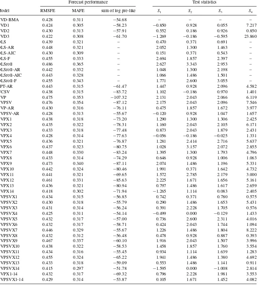
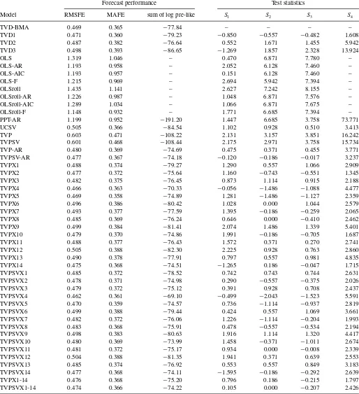
Tables 1 and2 present the results of our forecasting exer-cise for one quarter and one year ahead forecasts, respectively. Predictive likelihoods, MAFEs, and RMSFEs are telling a very similar story and it is one which says that the TVD models forecast very well. The main methods that occasionally forecast better are parsimonious TVP regression models which include only one regressor. For instance one year ahead, a TVP regres-sion model using two AR lags and housing starts as regressors forecasts slightly better than the TVD models. However, a pri-ori, a researcher in this field would not know which regressor to include (e.g., housing starts might not come to mind as being the logical regressor to include and the more logical choice of the unemployment rate does not yield a good forecast performance) and it might have been difficult to discover the fact that this was a good forecasting model using traditional model selection pro-cedures. An alternative to the use of TVD models would be to do sequential hypothesis testing procedures to try and select which regressors to include in a forecasting model. However, even in a constant coefficient model, pretesting problems would make this a risky strategy. In TVP regression models, such problems would worsen. Furthermore, the TVD model allows for a regres-sor to be included at some points in time, but excluded at others, which is not possible with a conventional testing strategy. In sum, TVD models are always among the top forecasting models in Tables1and2. Even in the cases where they are not the very best, it is hard to imagine a simple strategy that the researcher could use to reliably find the best forecasting model among the choices we consider. The best alternative appears to be simple averaging of parsimonious TVP models. In the remainder of this section we expand on these points.
TVD methods consistently forecast better than any of the OLS methods we consider. At the quarterly forecast horizon, forecast gains are small but at the annual horizon they are much larger. This holds true for simple AR forecasts, OLS methods using many predictors and factor methods. It also holds true regard-less of whether we use rolling or expanding windows of data to produce the OLS estimates. In general, we are finding evidence that constant coefficient models (even if estimated using rolling windows) do not forecast as well as TVD models which explic-itly allow for parameter change and change in model dimension over time.
The tables also show that nonparsimonious TVP models fore-cast very poorly as well. TVP regression models which include all the 14 predictors forecast poorly in our application. In theory, one might expect such a TVP model to be able to approximate a TVD model (i.e., the coefficients in the TVP model could evolve to be close to zero for a particular predictor and, thus, it
364 Journal of Business & Economic Statistics, July 2012
Table 1. Measures of one quarter ahead forecast performance
Forecast performance Test statistics
Model RMSFE MAFE sum of log pre-like S1 S2 S3 S4
TVD-BMA 0.428 0.311 −54.68 – – – –
TVD1 0.424 0.305 −58.23 −0.850 0.928 0.055 7.217
TVD2 0.430 0.313 −57.91 0.552 0.186 0.926 0.850
TVD3 0.422 0.308 −61.70 −1.269 −0.186 −0.595 23.860
OLS 0.439 0.321 – 0.470 0.371 0.691 –
OLS-AR 0.448 0.321 – 2.052 1.300 1.463 –
OLS-AIC 0.430 0.309 – 0.151 0.371 0.543 –
OLS-F 0.455 0.333 – 2.694 1.857 2.397 –
OLSroll 0.486 0.365 – 2.627 3.343 2.953 –
OLSroll-AR 0.442 0.332 – 1.048 1.300 2.198 –
OLSroll-AIC 0.443 0.328 – 1.066 1.486 1.501 –
OLSroll-F 0.455 0.343 – 1.771 2.600 3.055 –
PPT-AR 0.443 0.315 −61.47 1.447 0.928 2.096 4.582
UCSV 0.438 0.315 −83.72 1.102 −0.186 0.970 1.401
TVP 0.475 0.353 −107.32 2.131 2.043 2.066 6.119
TVPSV 0.476 0.354 −87.12 2.175 2.043 2.096 7.546
TVP-AR 0.430 0.316 −76.11 0.475 1.857 1.672 3.977
TVPSV-AR 0.428 0.313 −55.67 −0.120 0.928 1.047 1.657
TVPX1 0.438 0.318 −73.20 1.290 1.300 1.306 2.425
TVPX2 0.435 0.322 −78.31 1.160 2.043 2.105 6.171
TVPX3 0.433 0.318 −77.48 0.873 2.043 1.879 2.431
TVPX4 0.428 0.314 −77.63 −0.056 −0.186 −0.025 1.331
TVPX5 0.436 0.321 −76.87 1.281 2.414 2.716 5.637
TVPX6 0.437 0.323 −80.75 1.028 3.157 2.072 2.855
TVPX7 0.448 0.330 −83.24 1.395 1.300 1.793 4.796
TVPX8 0.433 0.314 −74.29 0.646 0.928 1.006 1.063
TVPX9 0.473 0.340 −87.11 2.074 1.486 1.196 5.331
TVPX10 0.442 0.324 −80.46 1.991 0.371 1.642 4.732
TVPX11 0.441 0.321 −69.65 1.572 2.785 2.179 3.000
TVPX12 0.461 0.331 −85.63 2.225 1.671 1.656 5.161
TVPX13 0.436 0.321 −80.94 0.797 1.486 1.617 2.659
TVPX14 0.418 0.302 −71.94 −1.265 1.114 0.083 2.405
TVPSVX1 0.434 0.315 −56.85 0.742 0.371 0.780 0.575
TVPSVX2 0.430 0.318 −55.79 0.290 1.486 1.653 5.431
TVPSVX3 0.431 0.314 −56.24 0.391 2.228 1.705 0.576
TVPSVX4 0.425 0.311 −54.14 −0.499 0.000 −0.129 1.433
TVPSVX5 0.432 0.317 −57.00 0.736 2.600 2.311 4.016
TVPSVX6 0.432 0.317 −58.71 0.424 2.043 1.744 1.094
TVPSVX7 0.446 0.329 −55.67 1.226 1.486 1.804 8.222
TVPSVX8 0.432 0.312 −56.48 0.478 0.928 0.887 0.393
TVPSVX9 0.467 0.337 −60.10 1.916 2.043 1.507 3.996
TVPSVX10 0.438 0.322 −58.53 1.458 1.857 1.760 3.554
TVPSVX11 0.434 0.316 −55.45 0.934 1.114 1.639 1.283
TVPSVX12 0.455 0.324 −65.22 1.941 1.486 1.380 4.692
TVPSVX13 0.433 0.318 −59.09 0.553 1.486 1.141 0.911
TVPSVX14 0.415 0.297 −51.78 −1.595 0.000 −1.008 2.814
TVPX1-14 0.432 0.317 −69.32 0.796 2.228 1.981 3.553
TVPSVX1-14 0.429 0.314 −53.87 0.105 1.671 1.452 4.082
could drop out of the model ensuring a dimension reduction). In practice, this is not happening and TVD models are forecasting better than TVP models.
TVD is also forecasting better than the popular structural break model of Pesaran, Pettenuzzo, and Timmerman (2006). The tables only present results for an AR version of this struc-tural break model. Including all the predictors leads to much worse forecast performance.
Our three TVD models exhibit similar forecast performance. Forecast metrics based on point forecasts indicate that TVD1 is the best, whereas predictive likelihoods indicate TVD2. How-ever, overall there is some evidence that use of BMA is beneficial in improving forecast performance since TVD-BMA exhibits strong forecast performance by both metrics.
Another class of popular forecasting models are parsimonious TVP models such as TVP-AR models. For instance, the popular
Table 2. Measures of one year ahead forecast performance
Forecast performance Test statistics
Model RMSFE MAFE sum of log pre-like S1 S2 S3 S4
TVD-BMA 0.469 0.365 −77.84 – – – –
TVD1 0.471 0.360 −79.23 −0.850 −0.557 −0.482 1.608
TVD2 0.487 0.382 −76.64 0.552 1.671 1.455 5.942
TVD3 0.498 0.393 −86.65 −1.269 1.857 2.328 13.924
OLS 1.319 1.046 – 0.470 6.871 7.780 –
OLS-AR 1.193 0.958 – 2.052 6.128 7.460 –
OLS-AIC 1.193 0.957 – 0.151 6.128 7.460 –
OLS-F 1.215 0.969 – 2.694 5.942 7.394 –
OLSroll 1.435 1.141 – 2.627 7.242 8.155 –
OLSroll-AR 1.226 0.987 – 1.048 6.871 7.576 –
OLSroll-AIC 1.289 1.034 – 1.066 6.871 7.675 –
OLSroll-F 1.148 0.932 – 1.771 6.685 7.394 –
PPT-AR 1.199 0.952 −191.20 1.447 6.685 3.758 73.771
UCSV 0.505 0.366 −84.54 1.102 0.928 0.510 3.413
TVP 0.603 0.471 −108.22 2.131 3.157 3.851 16.242
TVPSV 0.601 0.468 −108.44 2.175 2.971 3.758 15.734
TVP-AR 0.480 0.369 −74.69 0.475 0.371 0.455 3.771
TVPSV-AR 0.477 0.367 −74.18 −0.120 −0.186 −0.017 3.237
TVPX1 0.488 0.374 −79.27 1.290 0.557 1.066 2.909
TVPX2 0.477 0.372 −75.64 1.160 −0.743 −0.551 1.345
TVPX3 0.482 0.375 −76.45 0.873 1.114 0.915 2.188
TVPX4 0.466 0.363 −70.33 −0.056 −1.486 −1.088 4.477
TVPX5 0.469 0.358 −74.89 1.281 −1.486 −1.127 2.359
TVPX6 0.496 0.386 −80.42 1.028 0.000 1.044 2.579
TVPX7 0.493 0.377 −77.59 1.395 −0.186 −0.259 2.065
TVPX8 0.485 0.369 −76.24 0.646 0.000 −0.410 2.462
TVPX9 0.499 0.384 −81.41 2.074 1.486 1.339 5.401
TVPX10 0.479 0.370 −74.86 1.991 −0.186 −0.705 1.687
TVPX11 0.488 0.377 −76.43 1.572 0.371 0.270 2.741
TVPX12 0.505 0.388 −82.30 2.225 0.928 0.763 2.860
TVPX13 0.490 0.378 −77.91 0.797 0.557 0.981 4.835
TVPX14 0.475 0.368 −74.51 −1.265 0.186 −0.047 1.715
TVPSVX1 0.485 0.372 −78.52 0.742 0.743 0.744 2.631
TVPSVX2 0.478 0.371 −74.98 0.290 −0.557 −0.375 2.026
TVPSVX3 0.479 0.372 −75.12 0.391 0.928 0.708 2.437
TVPSVX4 0.462 0.361 −69.10 −0.499 −2.043 −1.523 5.591
TVPSVX5 0.470 0.359 −74.57 0.736 −1.114 −0.937 2.819
TVPSVX6 0.499 0.388 −79.44 0.424 0.557 1.069 3.661
TVPSVX7 0.482 0.372 −76.06 1.226 −1.114 −0.204 1.993
TVPSVX8 0.483 0.368 −75.91 0.478 −0.557 −0.534 2.194
TVPSVX9 0.498 0.383 −80.63 1.916 1.114 1.320 4.417
TVPSVX10 0.480 0.369 −73.99 1.458 −0.371 −1.011 2.674
TVPSVX11 0.481 0.372 −75.17 0.934 0.000 −0.008 2.339
TVPSVX12 0.504 0.388 −81.35 1.941 0.371 0.639 2.553
TVPSVX13 0.485 0.374 −76.92 0.553 0.557 0.849 3.183
TVPSVX14 0.477 0.368 −74.11 −1.595 −0.186 −0.292 2.639
TVPX1-14 0.476 0.368 −75.20 0.796 0.186 −0.215 1.797
TVPSVX1-14 0.474 0.366 −74.22 0.105 0.000 −0.207 2.426
UCSV model of Stock and Watson (2007) is a TVP regres-sion model with only a time-varying intercept (and stochastic volatility). The UCSV and TVPSV-AR model does forecast quite well, although overall TVD-BMA forecasts slightly bet-ter (see, in particular, the predictive likelihoods for one-quarbet-ter ahead forecasts).
Tables 1 and 2 also indicate the importance of allowing for stochastic volatility. This is not so clear in terms of point
forecasts, where homoscedastic and heteroscedastic versions of a model tend to have similar MAFEs and RMSFEs. However, predictive likelihoods in many cases, increase substantially when stochastic volatility is added to a model.
Tables1 and2 also present results for the four hypothesis tests of equal predictive performance described above (see also the online appendix). Remember that these are implemented so that each model is compared to the TVD-BMA model. Critical
366 Journal of Business & Economic Statistics, July 2012
values for the test statisticsS1,S2, andS3can be obtained from the standard normal distribution with positive values for test statistics indicating that TVD-BMA is forecasting better than the comparator model. Critical values forS4are obtained from theχ2(3) distribution.
Results from these tests are largely supportive of our previ-ous conclusions. That is, the value of these test statistics almost always indicates that TVD-BMA is forecasting better and it is often the case that this forecast improvement is statistically significant. For instance, the hypothesis of equal predictability between TVP models containing all the regressors and TVD-BMA is always rejected. In most cases, the same conclusion holds for the OLS methods. Tests of equal predictability be-tween TVD-BMA and parsimonious TVP models yield weaker results. Often it is the case that TVD-BMA forecasts better than a particular parsimonious TVP model at the 5% level of signifi-cance, but it is more common for the test statistics to be positive but insignificant at the 5% level. Although it is worth noting that there are many cases where TVD-BMA would forecast significantly better if we used a 10% level of significance.
Tables1 and2establish that, overall, the TVD approaches do tend to forecast better than many commonly used bench-marks. However, they relate to average forecast performance from 1980Q1 through the end of the sample. Rolling sums of log predictive likelihoods and square roots of rolling averages of forecast errors squared for one-quarter ahead and one-year ahead forecasts can be used to investigate how forecasting per-formance changes over time. Graphs of these are available in the online appendix. The most striking thing these graphs show is the deterioration in forecast performance around the time of the financial crisis. Unsurprisingly, this occurs with every fore-casting method. However, this deterioration is much less for the TVD methods than for some of the other methods. At the quar-terly forecast horizon, the forecasting superiority of TVD im-provements in forecast performance only appears after the early 1990s. In fact, there is a period in the 1980s and early 1990s that the over-parameterized TVP models (which include all the regressors) forecast better than the other models. However, later in the sample there is a clear deterioration in forecast perfor-mance of TVP and TVPSV. At the annual forecast horizon, this pattern is not found. The TVP regression models forecast poorly from the very beginning of our forecast period.
4. CONCLUSIONS
In this article, we have presented a battery of theoretical and empirical arguments for the potential benefits of TVD models. Like TVP models, TVD models allow for the values of the parameters to change over time. Unlike TVP models, they also allow for the dimension of the parameter vector to change over time. Given the potential benefits of a TVD framework, the task is to build specific TVD models. This task was taken up in Section2of this article where three different TVD models were developed. All these models are dynamic mixture models and, thus, have the enormous benefit that we can draw on existing methods of posterior computation developed in Gerlach, Carter, and Kohn (2000).
An empirical illustration involving forecasting US inflation illustrated the feasibility and desirability of the TVD approach.
SUPPLEMENTAL MATERIAL
The online appendix, which accompanies this paper, is also available athttp://personal.strath.ac.uk/gary.koop/research.htm.
ACKNOWLEDGMENTS
Koop, Leon-Gonzalez, and Strachan are Fellows of the Rimini Centre for Economic Analysis. We would like to thank the Economic and Social Research Council and the Australian Research Council for financial support under Grant RES-062-23-2646 and Grant DP0987170, respectively. Contact address: Gary Koop, Department of Economics, Strathclyde University, Glasgow, G4 0GE, United Kingdom.
[Received May 2010. Revised January 2012.]
REFERENCES
Amato, J., and Swanson, N. (2001), “The Real-Time Predictive Content of Money for Output,”Journal of Monetary Economics, 48, 3–24. [358] Ang, A., Bekaert, G., and Wei, M. (2007), “Do Macro Variables, Asset Markets,
or Surveys Forecast Inflation Better?”Journal of Monetary Economics, 54, 1163–1212. [361,363]
Ballabriga, F., Sebastian, M., and Valles, J. (1999), “European Asymmetries,”
Journal of International Economics, 48, 233–253. [360]
Banbura, M., Giannone, D., and Reichlin, L. (2010), “Large Bayesian Vector Autoregressions,”Journal of Applied Econometrics, 25, 71–92. [361] Bauwens, L., Koop, G., Korobilis, D., and Rombouts, J. (2011), “The
Con-tribution of Structural Break Models to Forecasting Macroeconomic Time Series,” Rimini Centre for Economic Analysis, working paper, 11–38. [362] Canova, F. (1993), “Modelling and Forecasting Exchange Rates Using a Bayesian Time Varying Coefficient Model,”Journal of Economic Dynamics and Control, 17, 233–262. [358]
——— (2007),Methods for Applied Macroeconomic Research, Princeton: Princeton University Press. [360]
Canova, F., and Ciccarelli, M. (2004), “Forecasting and Turning Point Pre-dictions in a Bayesian Panel VAR Model,”Journal of Econometrics, 120, 327–359. [360]
Carter, C., and Kohn, R. (1994), “On Gibbs Sampling for State Space Models,”
Biometrika, 81, 541–553. [361]
Chan, J. C. C., and Jeliazkov, I. (2009), “Efficient Simulation and Integrated Likelihood Estimation in State Space Models,”International Journal of Mathematical Modelling and Numerical Optimisation, 1, 101–120. [361] Chib, S., and Greenberg, E. (1995), “Hierarchical Analysis of SUR Models
With Extensions to Correlated Serial Errors and Time-Varying Parameter Models,”Journal of Econometrics, 68, 339–360. [360]
Ciccarelli, M., and Rebucci, A. (2002), “The Transmission Mechanism of Euro-pean Monetary Policy: Is There Heterogeneity? Is It Changing Over Time?,” International Monetary Fund working paper, WP 02/54. [360]
Cogley, T., and Sargent, T. (2005), “Drifts and Volatilities: Monetary Policies and Outcomes in the post WWII U.S.,”Review of Economic Dynamics, 8, 262–302. [358,363]
D’Agostino, A., Gambetti, L., and Giannone, D. (2009), “Macroeconomic Forecasting and Structural Change,” ECARES working paper 2009–2020. [358,361]
De Mol, C., Giannone, D., and Reichlin, L. (2008), “Forecasting Using a Large Number of Predictors: Is Bayesian Shrinkage a Valid Alternative to Principal Components?,”Journal of Econometrics, 146, 318–328. [361]
Diebold, F., and Mariano, R. (1995), “Comparing Predictive Accuracy,”Journal of Business Economics and Statistics, 13, 134–144. [362]
Durbin, J., and Koopman, S. (2002), “A Simple and Efficient Simulation Smoother for State Space Time Series Analysis,”Biometrika, 89, 603–616. [361]
George, E., Sun, D., and Ni, S. (2008), “Bayesian Stochastic Search for VAR Model Restrictions,”Journal of Econometrics, 142, 553–580. [361] Gerlach, R., Carter, C., and Kohn, R. (2000), “Efficient Bayesian Inference in
Dynamic Mixture Models,”Journal of the American Statistical Association, 95, 819–828. [359,360,361,366]
Geweke, J., and Amisano, G. (2011), “Hierarchical Markov Normal Mixture Models With Applications to Financial Asset Returns,”Journal of Applied Econometrics, 26, 1–29. [362]
Giacomini, A., and White, H. (2006), “Tests of Conditional Predictive Ability,”
Econometrica, 74, 1545–1578. [362]
Giordani, P., and Kohn, R. (2008), “Efficient Bayesian Inference for Multiple Change-Point and Mixture Innovation Models,”Journal of Business and Economic Statistics, 12, 66–77. [359]
Giordani, P., Kohn, R., and van Dijk, D. (2007), “A Unified Approach to Non-linearity, Structural Change and Outliers,”Journal of Econometrics, 137, 112–133. [359]
Groen, J., Paap, R., and Ravazzolo, F. (2010), “Real-Time Inflation Forecasting in a Changing World,”Federal Reserve Bank of New York Staff Report Number 388. [358,361]
Kim, S., Shephard, N., and Chib, S. (1998), “Stochastic Volatility: Likelihood Inference and Comparison With ARCH Models,”Review of Economic Stud-ies, 65, 361–393. [361,363]
Koop, G. (2003),Bayesian Econometrics, Chichester: Wiley. [361]
Koop, G., and Korobilis, D. (2012), “Forecasting Inflation Using Dynamic Model Averaging,”International Economic Review, forthcoming. [358,361] Koop, G., Le´on-Gonz´alez, R., and Strachan R. W. (2009), “On the Evolution of the Monetary Policy Transmission Mechanism,”Journal of Economic Dynamics and Control, 33, 997–1017. [359,361]
Koop, G., Le´on-Gonz´alez, R., and Strachan R. W. (2010), “Dynamic Probabil-ities of Restrictions in State Space Models: An Application to the Phillips Curve,”Journal of Business and Economic Statistics, 28, 370–379. [358]
Koop, G., and Potter, S. (2011), “Time Varying VARs With Inequality Restric-tions,”Journal of Economic Dynamics and Control, 35, 1126–1138. [359] Korobilis, D. (2012), “VAR Forecasting Using Bayesian Variable Selection,”
Journal of Applied Econometrics, forthcoming. [361]
Pesaran, M. H., Pettenuzzo, D., and Timmerman, A. (2006), “Forecasting Time Series Subject to Multiple Structural Breaks,”Review of Economic Studies, 73, 1057–1084. [362,364]
Primiceri, G. (2005), “Time Varying Structural Vector Autoregressions and Monetary Policy,”Review of Economic Studies, 72, 821–852. [358,361,363] Raftery, A., Karny, M., Andrysek, J., and Ettler, P. (2010), “Online Prediction Under Model Uncertainty via Dynamic Model Averaging: Application to a Cold Rolling Mill,”Technometrics, 52, 52–66. [361]
Staiger, D., Stock, J., and Watson, M. (1997), “The NAIRU, Unemploy-ment and Monetary Policy,”Journal of Economic Perspectives, 11, 33–49. [358]
Stock, J., and Watson, M. (2007), “Why has US Inflation Become Harder to Forecast?,”Journal of Money, Credit and Banking, 39, 3–33. [362,365] Stock, J., and Watson, M. (2009), “Phillips Curve Inflation Forecasts,” in
Un-derstanding Inflation and the Implications for Monetary Policy, eds., J. Fuhrer, Y. Kodrzycki, J. Little, and G. Olivei, Cambridge: MIT Press, ch. 3, pp. 99–202. [358,361,362,363]
Stock, J., and Watson, M. (2010), “Modeling Inflation After the Crisis,” National Bureau of Economic Research, working paper #16488. [358]