www.elsevier.com/locate/dsw
Comparison of probability measures: Dominance of the
third degree
Lars Thorlund-Petersen
∗Department of Operations Managements, Copenhagen Business School, Solbjerg Pl. 3, DK-2000 Frederiksberg, Denmark
Received 1 August 1997; received in revised form 1 March 2000
Abstract
This note provides necessary and sucient conditions for third-degree stochastic dominance between the probability measures on a nite grid ofnpoints. Verifying these conditions involvenlinear andnquadratic inequalities; the arithmetic operation of division is not required. The results are compared with those of Fishburn and Lavalle, Math. Operat. Res. 20 (1995) 513–525 and Milne and Neave, Management Sci. 40 (1994) 1343–1352. Finally, the solution to an open problem in Fishburn and Lavalle, Math. Operat. Res. 20 (1995) 513–525 is presented. c 2000 Elsevier Science B.V. All rights reserved.
Keywords:Decision theory; Stochastic dominance; Third-degree dominance
1. Introduction
Stochastic-dominance rules are widely used in analysis of decision making under risk or uncertainty, see, e.g., Ref. [3]. Such rules are dened by partial specication of the decision maker’s preferences. In the usual framework of the expected-utility model and unidimensional random incomes or payos, dominance of the rst degree corresponds to the assumption that more income is preferred to less; dominance of the second degree corresponds to the stronger assumption that the decision maker in addition is risk averse. In many applications further restrictions on preferences are assumed, such as “aversion to downside risk”, see Ref. [4]. This assumption corresponds to the dominance of the third degree dened in Ref. [9], which is necessary for the dominance of any higher degree. For example, by considering the dominance of the third degree and
∗Also at: Bodo=Graduate School of Business, N-8002 Bodo=, Norway.
Correspondence address:Copenhagen Business School, Department of Operations Management, Solbjerg Pl. 3, DK-2000 Frederiksberg, Denmark.
E-mail address: [email protected] (L. Thorlund-Petersen).
beyond, Ritchken and Kuo in Ref. [6] have obtained stronger option-pricing bounds than those of (simple) risk aversion.
In the following, suppose that N ={1;2; : : : ; n} is a given nite set of states of the world. Correspond-ingly, let x = (x1; : : : ; xn); y = (y1; : : : ; yn) be n-vectors of random income and p = (p1; : : : ; pn); q =
(q1; : : : ; qn) be probability measures on 2N, thus pi; qi¿0; PNpi = PNqi = 1. Furthermore, let U be a
given set of functions on the real line. Then (y; q) (stochastically)dominates(x; p) with respect toU if and only if
n X
i=1
u(xi)pi6 n X
i=1
u(yi)qi; for allu∈U: (1)
Predominantly, three classes of utility functions commonly studied in the literature are considered here. Let
U1 be the class of increasing functions, U2⊂U1 the subclass of concave functions, and U3⊂U2 the fur-ther subclass of functions having a convex derivative. If U equals U1; U2, or U3, then dominance with
respect to U is called dominance of the rst, second, or third degree, respectively. The third degree gen-erally is more dicult to analyse than the rst and second degree and it is of interest to consider spe-cial cases such as random incomes being conned to a nite set of equally spaced points as in Refs. [2,5].
Therefore, consider in (1) the casex=y andx2−x1=· · ·=xn−xn−1¿0. Without loss of generality, it is
furthermore assumed throughout that x= (1;2; : : : ; n), thus all possible incomes xi lie in the grid {1;2; : : : ; n}.
This distributional assumption may be interpreted as an approximation of a more general framework, for example, such an approximation argument is implicit in Ref. [6]. On the other hand, in some cases only integer values are relevant, hence the grid assumption follows naturally as for example in Ref. [8].
Given the above assumptions, (1) denes a dominance relation on the given set of probability measures. Thus dominance of p by q with respect to U means that
n X
i=1
u(i)ti60 for allu∈U; (2)
wheret=p−q. For U=U; = 1;2;3; let C denote the convex cone of directions t for which P Nti= 0
and (2) holds. Clearly, t∈C entails that the mean Et=P
Niti satises Et60.
Necessary and sucient conditions for rst- and second-degree dominance follows from Refs. [2,5]: q
dominates p of the rst or second degree if and only ift=p−q for k= 1; : : : ; n−1 satises
k X
i=1
ti¿0 (3a)
or
k X
i=1
(k+ 1−i)ti¿0; (3b)
respectively. Accordingly, if P
Nti= 0, then t ∈ C1 or t ∈ C2 if and only if t satises (3a) or (3b). In
particular, C1 andC2 are nite cones for any n.
and stochastic dominance has so far not been fully explored in the literature. This note contains a complete characterization for the third degree, in terms of necessary and sucient conditions for a given dierence
t=p−q determining a direction of the cone C3.
The main result on third-degree dominance is given in Section 2, followed by numerical examples in Section 3. In Section 4 the extreme directions of the cone C3 are discussed and in Section 5 the results of Section 2
are used to solve an open problem in Ref. [2].
The present characterization of third-degree dominance is possible basically due to the following simple geometric property of the graph of a quadratic function. Consider real numbersA; B; C whereA6= 0, and letf
be the quadratic functionf()=A2+B+C. For given, letL()=f′() (−)+f()=(2A+B)−A2+C
denote the ane approximation (or tangent) off at. It is a simple exercise to show that for any two points
¡ , the equality L() =L() holds if and only if bisects the interval [; ]; = (+)=2. In summary,
a quadratic function has the tangential bisection property.
2. Third-degree dominance
In studying third-degree stochastic dominance, one encounters the diculty that the cone C3 fails to be nite for n¿4. In spite of this, there exists a rather simple set of conditions for t ∈C3 which is in nature
quadratic. First, for k= 1; : : : ; n−1 dene the linear form in t1; : : : ; tk−1 by
Vk(t) = k−1
X
i=1
(k−i+ 1)(k−i)ti; (4)
whereV1(t) = 0. Secondly, for k= 1; : : : ; n let Dk(t) denote the quadratic form in t1; : : : ; tk determined by the k×k matrix −2[(i−j)2]k
i; j=1,
Dk(t) =−2 k X
i=1
k X
j=1
(i−j)2titj; (5)
thus, D1(t) = 0; D2(t) =−4t1t2.
The main result can now easily be stated. If Et60, t ∈C3 if and only if the largest of the two numbers
Vk(t); −Dk(t) is nonnegative for k= 2; : : : ; n−1 (see Theorem 1). However, some further concepts must be
introduced before Theorem 1 can be proved.
It suces to check (2) against functions u which generate an extreme direction in U3. These directions
are well known to be determined by the functions of the following form. For every real number , dene
u() =−(−)2 if 6 andu() = 0 otherwise; for=∞, deneu() =. Thus, in order fort∈C3 to
hold, (2) must be satised for every such function u.
For givenn-vector t, dene the function ft on the real line by ft() =−PNu(i)ti. It is readily seen that
for any k∈ {1; : : : ; n−1}, one has
ft() =
0; 61;
(−1)2t1+ (−2)2t2+· · ·+ (−k)2tk; k ¡ 6k+ 16n;
(−1)2t1+ (−2)2t2+· · ·+ (−n)2tn; n ¡ :
(6)
The piecewise quadratic functionft consists of at mostn+1 pieces determined by the subdivision−∞;1;2; : : : ; n;∞of the real line. Furthermore,ft has a piecewise ane derivativeft′at every and a second derivativeft′′
for ¿1:
1
2ft′() = (
(−1)t1+ (−2)t2+· · ·+ (−k)tk; k ¡ 6k+ 16n;
−Et; n ¡ ; (7)
1
2ft′′() =t1+t2+· · ·+tk; k ¡ ¡ k+ 16n: (8)
It is useful to consider some examples. Firstly, ift= (1;−1;0; : : : ;0)∈C1, then f
t is convex for 1¡ 62
and ane for ¿2. Secondly, if t= (1;−2;1;0; : : : ;0)∈C2, then f
t is convex for 1¡ 62, concave for
2¡ 63, and constant for ¿3. Thirdly, for t= (1;−3;3;−1;0; : : : ;0)∈C3; f
t is convex–concave–convex
on 1¡ 62; 2¡ 63; 3¡ 64 and zero for ¿4. Furthermore,ft is symmetric at = 2:5 andft()¿0
if and only if 1¡ ¡4.
Dominance of the rst, second, and third degree can conveniently be expressed in terms of conditions on
ft. It follows from (3), (7), and (8) that whenever PNti= 0, then t ∈C2 (or t ∈ C1) if and only if the
function ft is nonnegative and increasing (or nonnegative, increasing, and convex). Since it suces to check
(2) against the functions u, then t∈C3 holds if and only if ft is nonnegative.
The remaining part of this section is organized as follows. Firstly, for every function ft, an auxiliary
function ˆft is dened and analysed. This function has the important property that it being nonnegative is equivalent to third-degree partial-sums dominance. Secondly, it turns out that in order to test nonnegativity of
ft, it suces to consider for which ˆft()¡0. In this manner the exact relationship between the dominance
and partial-sums dominance is established.
2.1. Third-degree partial-sums dominance and the functionfˆt
For any ft in (6), the function ˆft is dened as follows. The ane approximation of ft at any integer j is
given byLj(;t)=ft′(j)(−j)+f(j). If ¡1 orn ¡ , then dene ˆft()=ft() and for 16k ¡ 6k+16n,
dene
ˆ
ft() =
(
max{Lk(;t); Lk+1(;t)}; t1+· · ·+tk¿0;
min{Lk(;t); Lk+1(;t)}; t1+· · ·+tk¡0:
(9)
By (9), ˆft is piecewise ane and ˆft(k) =ft(k) for k∈ {1; : : : ; n}. The number ˆ is called an inection point
of ˆft if for any ¿0; fˆt is nonane on [ ˆ−;ˆ+]. Recall from Section 1 that any quadratic function has the tangential bisection property. Therefore, the function ˆft is piecewise ane with respect to a particularly neat subdivision.
Lemma 1. The set of inection points offˆt is contained in {k+ 1=2|k= 1; : : : ; n−1} and the value offˆt at any possible inection point k+ 1=2 equalsVk(t) dened in (4).
Proof. First, assume for given k∈ {1; : : : ; n−1} that 2(t1+· · ·+tk) =ft′(k+ 1)−ft′(k)6= 0, hence, ft is
quadratic and nonane on the interval [k; k+ 1]. Then there exists ˆk ∈]k; k+ 1[, uniquely determined by Lk( ˆk;t) =Lk+1( ˆk;t), hence ˆk−k= (ft′(k+ 1)−ft(k+ 1) +ft(k))=2(t1+· · ·+tk) =12, the latter equality by
(6) and (7). Secondly, ift1+· · ·+tk= 0, then ˆft() =ft() is ane on ∈[k; k+ 1]. This proves that ˆft has at
mostn−1 inection pointsk+12; k= 1; : : : ; n−1. Finally, ˆft (k+12) =Lk (k+12;t) = ( 1
As an example, if n= 5, then ˆft is nonnegative if Vk(t)¿0 for k= 2;3;4 and −Et¿0, thus,
hence, partial-sums dominance holds by Refs. [2,5]. In general, one has
Proposition 1. Let p; q be given probability measures and t=p−q. Then q third-degree partial-sums dominates pif and only if the auxiliary functionfˆt is nonnegative; a property which again is equivalent to
(10):
V2(t); : : : ; Vn−1(t);−Et¿0: (10)
Proof. By Lemma 1, the piecewise ane function ˆft is nonnegative if and only if (10) holds. Furthermore, (10) is equivalent to conditions for third-degree partial-sums dominance in Refs. [2,5].
2.2. Third-degree dominance and the functions ft ,fˆt
If 16k ¡ 6k+ 16n, then by (6)
ft() = (t1+t2+· · ·+tk)2−2(t1+ 2t2+· · ·+ktk)+ (t1+ 4t2+· · ·+k2tk):
The discriminant of this second-degree polynomial in is by denition:
4(t1+ 2t2+· · ·+ktk)2−4(t1+t2+· · ·+tk)(t1+ 4t2+· · ·+k2tk): (11)
The characterization of third-degree dominance can now be proved.
Theorem 1. Letp; qbe given probability measures andt=p−q.Thenqthird-degree stochastically dominates
p if and only if the function ft is nonnegative; a property which again is equivalent to
max{Vk(t);−Dk(t)}¿0; k= 2; : : : ; n−1; (13a)
−Et¿0: (13b)
Proof. Equivalence of third-degree dominance and nonnegativity of ft has already been established. Thus,
suppose that ft is nonnegative. Clearly (13b) holds. If Vk(t)¡0 for some k= 2; : : : ; n−1, then as ft is
quadratic on the interval [k; k + 1] and ft(k); ft(k+ 1)¿0, it follows that ft′(k)606f′t(k+ 1), see (9).
Therefore, ft is quadratic, convex, and nonnegative on this interval. Thus, by Lemma 2, it must be the case
Table 1
35tk 14 −27 0 21 0 0 −8
Vk(35t) 0 28 30 6 −2 3 ∗
Dk(35t) 0 1512 1512 0 0 0 576
Table 2
tk 0.5 −1:75 3.5 −2:25
Vk(t) 0 1 −0:5 ∗
Dk(t) 0 3.5 0 9
On the other hand, suppose that (13) holds. Then Et60 and ft is nonnegative outside the interval [1; n].
If ft attains its global minimum at ∗∈[k; k+ 1]⊂[1; n] andft(∗)¡0, then k¿2 and ft is quadratic and
convex on [k; k+ 1], hence, by Lemma 2, Vk(t)¡0¡ Dk(t); this contradicts (13a).
3. Examples
The analysis in Ref. [2] of partial-sums dominance is in part motivated by considerations of computational simplicity. By Proposition 1 and Theorem 1 it follows that third-degree stochastic dominance is almost as simple in this respect. In testing for third-degree dominance, one must in addition to the linear form Vk(t)
calculate the quadratic form Dk(t) and these calculations do not require the arithmetic operation of division
involving t. Note that Vn(t) is not dened (hence, the ∗ in Tables 1–5) and Dn(t) = 4(Et)2 as PNti= 0.
Theorem 1 is illustrated by two examples.
Example 1. Consider as in Ref. [2, p. 522], n= 7; p= (1435;0;0;2135;0;0;0); q= (0;2735;0;0;0;0;358). Then 35Et=−12, and fork= 1; : : : ;7, see Table 1.
As V5(t)¡0 and D5(t) = 0, partial-sums dominance fails by (10) whereas stochastic dominance holds by
(13). The smallest n for which this can happen is n= 4; if t= (0:5;−1:75;3:5;−2:25), then Et=−1:5, and for k= 1; : : : ;4, see Table 2.
Example 2. For∈[0;1] letpbe given by binomial probabilities on the grid {1; : : : ;7}; pi= ( n i−1)
i−1(1−
)7−i; i= 1; : : : ;7, and letq= (0;1
6; : : : ; 1
6) on {1; : : : ;7}. The choice between pandq has the following simple
economic interpretation. A decision maker who initially has riskless income 1 dollar faces the choice between the outcome in dollars equal to the number of heads from six successive tosses of a (possibly nonregular) coin, or receiving the dollar amount equal to the points resulting from a single throw of a die.
Clearly, if = 0, then q rst-degree dominates p= (1;0; : : : ;0). Using conditions (3a), (3b), or (13),
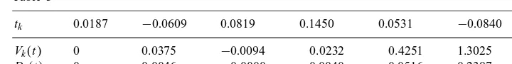
one nds that q rst-, second-, or third-degree dominates p if 60:4475; 60:4668, or 60:4846, respec-tively. For = 0:4846, binomial probabilities are p= (0:0187;0:1057;0:2486;0:3116;0:2197;0:0826;0:0130); Et=−0:5924, and fork= 1;2; : : : ;7, see Table 3.
Table 3
tk 0.0187 −0:0609 0.0819 0.1450 0.0531 −0:0840 −0:1537 Vk(t) 0 0.0375 −0:0094 0.0232 0.4251 1.3025 ∗ Dk(t) 0 0.0046 0.0000 −0:0040 −0:0516 0.2387 1.4038
4. Extreme directions
For n= 4, the cones C1 and C2 have a nite number of extreme directions determined by the columns of
the matrices
see Ref. [5]. The rst two columns of (14b) correspond to a mean-preserving spread as dened in Ref. [7] and the last column is a pure income decrease. While (14) can be generalized in a straightforward fashion to any n, the structure of C3 is more complicated. A complete characterization of extreme directions for any n
is beyond the scope of this note and only the cases n= 4;5;7 are discussed.
Any direction t has support {i|ti6= 0} and length max{j−i|ti; tj6= 0}. For C1 or C2 the largest length
of any extreme direction is 1 or 2, independently of n. Apparently, there is no similar upper bound for the length of extreme directions of C3. In order to determine extreme directions, the following lemma is needed.
Lemma 3. If s∗= (0; : : : ;0;1;−3;3;−1;0; : : : ;0)has support j; : : : ; j+ 36n;then f
s∗() equals zero outside
the interval ]j; j + 3[. If s is an extreme direction of C3 of length at least 4; then on every interval
]j; j+ 3[⊂[1; n]; fs(0) = 0holds for some 0 in this interval.
Table 4
sk 1 −3:5 7 −12 48 −76:5 36
Vk(s) 0 2 −1 5 −4 68 ∗
Dk(s) 0 14 0 96 0 9792 0
compare with (14). For n= 5, the following directions are extreme:
1− 0
−3 + 2+2 1−
3 + −3 + 2+2
−1−4−32 3 +
2+ 22 −1−2−2
; 06; 61; (16)
The mean of the rst column of (15) and the second one of (16) equals −2(1 +). The rst column of (16) has zero mean and length 4 if 0¡ ¡1. Furthermore, if 0¡ ; ¡1, then the rst column of (15) (for =1
2, see Table 2) and both columns of (16) dene directions inC
3 for which partial-sums dominance
does not hold.
Finally, if n= 7, then an extreme direction of length 6 and zero mean can be constructed as follows. For 0¡ ¡1 chooses1; s2; s3 by settings1= 1; s2= (−3 + 2+2)(1−)−1; s3= (3 +)(1−)−1. Thens1¿0,
D3(s) = 0,fs(3) = 4s1+s2¿0, fs(4) = 9s1+ 4s2+s3¿0 (see (16)). Chooses4 such that s1+s2+s3+s460,
fs(5) = 16s1+ 9s2+ 4s3+s4¿0, thus,s4 must satisfy −(1 + 3)2(1−)−1¡ s4 6−(1 +)2(1−)−1. Then
chooses5 such thatD5(s) = 0; by the iterative formula (12), this entails thats5 satises s4fs(4) +s5fs(5) = 0.
The construction is completed by determining s6; s7 such that s= (s1; : : : ; s7) satises P71si= 0 and Es= 0.
For =12 and s4=−12, the extreme direction s is shown in Table 4 for k= 1; : : : ;7.
Thus, under the assumption of a xed grid, there exist extreme directions of length larger than that of
s∗= (: : : ;1;−3;3;−1; : : :), in contradistinction to a related but dierent result in Ref. [1].
Generally, it is conjectured that for every odd n¿5 there exist extreme directions in C3 of zero mean and
length n−1.
5. The solution to an open problem in Ref. [2]
In Ref. [2, p. 523] the authors ask whether it is possible to have third-degree stochastic dominance and not partial-sums dominance of some higher degree. Due to the tangential bisection property of quadratic functions, inspection of the graphs of ft and ˆft provides the answer.
First, it follows from Ref. [2, Theorem 2] and (8) that for given measures p; q; t=p−q, and n¿5, q
fourth-degree partial-sums dominates p if and only if (17) holds:
k X
i=1
Vi(t)¿0; k= 2; : : : ; n−2; (17a)
Vn−1(t)¿0; (17b)
−Et¿0: (17c)
Table 5
tk 0 0.5 −1:75 3.5 −2:25
Vk(t) 0 0 1 −0:5 ∗
Dk(t) 0 0 3.5 0 9
To see this, consider t such that the function ft is nonnegative,t∈C3. Then by Lemma 1 the function ˆft
is ane on every interval [k−1=2; k+ 1=2]⊂[1; n] and nonnegative at =k, ˆft(k) =ft(k)¿0. Accordingly,
the values of ˆft at the endpoints on such intervals must satisfy ˆft(k−1
2) + ˆft(k+21) = 2 ˆft(k)¿0. Therefore,
it follows that if t∈C3, then
Vk−1(t) +Vk(t)¿0; k= 2; : : : ; n−1: (18)
If furthermore Et= 0, then ˆft must be nonnegative on [n−1; n] hence Vn−1(t)¿0. Thus, (17) follows from
(18).
In summary, third-degree dominance of p by q and E(p−q) = 0 implies fourth-degree partial-sums dominance as well. The provision of zero mean cannot in general be vaiwed; consider for example the second column of (16) with =1
2 which gives the simple variant of Table 2, for k= 1; : : : ;5, see Table 5.
As V4(t)¡0, (17b) is violated and hence fourth-degree partial-sums dominance does not hold.
Acknowledgements
The author has beneted from comments by E.H. Neave and critical remarks from an associate editor have resulted in several improvements.
References
[1] P.C. Fishburn, Moment-preserving shifts and stochastic dominance, Math. Oper. Res. 7 (1982) 629–634. [2] P.C. Fishburn, I.H. Lavalle, Stochastic dominance on unidimensional grids, Math. Oper. Res. 20 (1995) 513–525. [3] H. Levy, Stochastic dominance and expected utility: survey and analysis, Manage. Sci. 38 (1992) 555–593. [4] C. Menezes, C. Geiss, J. Tressler, Increasing downside risk, Amer. Econom. Rev. 70 (1980) 921–932. [5] F. Milne, E.H. Neave, Dominance relations among standardized variables, Manage. Sci. 40 (1994) 1343–1352.
[6] P. Ritchken, S. Kuo, On stochastic dominance and decreasing absolute risk averse option pricing bounds, Manage. Sci. 35 (1989) 51–59.
[7] M. Rotchschild, J. Stiglitz, Increasing risk: I. A denition, J. Econom. Theory 2 (1970) 225–243.
[8] W. Stanford, On comparing equilibrium and optimum payos in a class of discrete bimatrix games, Math. Social Sci. 39 (2000) 13–20.