ELECTRONIC COMMUNICATIONS in PROBABILITY
A MARTINGALE ON THE ZERO-SET OF A HOLOMORPHIC
FUNC-TION
PETER KINK
University of Ljubljana, Faculty of Computer and Information Science Trzaska cesta 25, SI-1001 Ljubljana, Slovenia.
email: [email protected]
SubmittedAugust 28, 2008, accepted in final formNovember 4, 2008 AMS 2000 Subject classification: Primary 60H30; secondary 60G46,60H10;
Keywords: complex martingales, stochastic differential equations, holomorphic functions
Abstract
We give a simple probabilistic proof of the classical fact from complex analysis that the zeros of a holomorphic function of several variables are never isolated and that they are not contained in any compact set. No facts from complex analysis are assumed other than the Cauchy-Riemann definition. From stochastic analysis only the Itô formula and the standard existence theorem for stochastic differential equations are required.
1
Introduction
It is well known that numerous facts from complex analysis can be given probabilistic proofs or interpretation, many of which stem from Paul Lévy’s striking observation that the image of a complex Brownian motion is simply a time changed complex Brownian motion. Itô calculus in particular seems to be well-suited for giving interesting insights into classical facts as well as being a tool for deriving new or refined results. We refer the reader to[Bas95] and the bibliography therein for some examples. In this article we give a probabilistic approach to analyzing the zero-set of a holomorphic function onCn(wheren≥2).
Here we use a stochastic differential equation (SDE) which has a strong solution that remains on the zero-set of a given holomorphic function of several variables. We then prove that the solution reaches any given radius with a strictly positive probability by computing the radial process and the gradient norm process. The novelty in this application of stochastic calculus seems to be the use of the gradient norm process and the fact that this process happens to be a submartingale along the solution to the equation (1).
In section 2 we introduce the notation and basic facts to be used. The formalism developed here is tailored to the specific situation, but the notions should be recognizable to anyone familiar with conformal martingales, see for instance [RY91]. In section 3 we state and prove the theorem. The main claim is a well known fact from complex analysis of several variables (see for instance [Kra92]or[Ran86]) and can be proved in several ways, but the probabilistic argument used here has apparently not been observed. The proof here also shows how to construct semimartingales
with desirable properties on analytic sets or complex manifolds without the use of local coordinates which are common in most literature on stochastic analysis on manifolds. Conceivably these kinds of SDE’s could be useful or interesting in other contexts. In the last section we conclude with a numerical illustration and remarks.
2
Preliminaries and notation
LetA andMl oc
c denote the space of continuous real valued processes with bounded total variation and the space of continuous real valued local martingales respectively. We use a complexification of the space ofR2valued semimartingales.
Definition 1. Acomplex semimartingaleS is aC-valued process of the form S=S0+X+iY =S0+A+M+i(B+N) where A,B∈ A and M,N∈ Ml oc
c are orthogonal local martingales with〈M,N〉=0and〈M〉=〈N〉. Let the space of complex semimartingales be denoted byQ.
Definition 2. Thecomplex covariationof a pair S1,S2∈ Qis defined to be theC-bilinear form
〈S1,S2〉:=〈X1+iY1,X2+iY2〉=〈X1,X2〉 − 〈Y1,Y2〉+i(〈X1,Y2〉+〈X2,Y1〉)
A pair S1,S2∈ Qof complex semimartingales areorthogonaliff their complex covariation is〈S1,S2〉= 0.
For the process Z = B1+iB2 whereB1 andB2 are orthogonal Brownian motions we therefore have〈Z,Z〉=2t.
Definition 3. The Itô integral of a complex valued process along a complex(Ft)-semimartingale is
Z t
0
(us+i vs)d(Xs+iYs):=
Zt
0
(usd Xs−vsd Ys) +i
Z t
0
(vsd Xs+usd Ys).
where u and v are(Ft)-adapted.
We note that complex orthogonality of two complex martingales does not require the orthogonal-ity of the corresponding real valued coordinate martingales, indeed, 〈S,S〉=〈S,S〉=0 for any complex semimartingale.
The bilinearity of the complex quadratic variation extends to complex integrals in the same way as it does in the real case. In particular, we make use of the following statements which are easily verified using the definitions above and basic properties for real semimartingales.
Proposition 1. Let f be an integrable (Ft)-adaptedC-valued process and S ∈ Q a complex semi-martingale (respectively semi-martingale). Then
Z
f dS
Let S1,S2∈ Qand let f and g be integrable(Ft)-adaptedC-valued processes. Then
In particular,R f dS andRg dS are orthogonal semimartingales,
〈
Proof. Compute the quadratic variations and covariations of the real and imaginary parts of the according functions and integrals.
the Itô formula takes the familiar form.
Theorem 1(Itô formula). For a twice differentiable complex function f :C→C
and a complex semimartingale S∈ Qwe have
f(S,S)−f(S0,S0) =
This generalizes to complex functions of severable variables. We need this generalization only for the case of two complex variables and orthogonal martingales and we write it out explicitly for the sake of clarity.
Theorem 2(Itô formula). Let f be a C2complex function of two complex variables f :C2→C
and let Z,W∈ Qbe orthogonal complex semimartingales. Then
f(Z,W)−f(Z0,W0) =
In the case of a holomorphic function this simplifies still further by the Cauchy-Riemann equations
Theorem 3(Itô formula). Let f be a holomorphic function of two variables and let Z,W ∈ Q be orthogonal complex semimartingales. Then
f(Z,W)−f(Z0,W0) =
Z
∂zf d Z+
Z
∂wf dW.
We shall also use the existence theorem for SDE for the case of bounded and Lipschitz coefficients. As a basic reference for all these facts we cite[RY91].
3
Statement and proof
In what follows we denote the complex derivative of a holomorphic function f byfz:=∂zf. Let N:={z∈Cn: f =0}
be the zero-set of f and let
D:={z∈Cn:|fz1|2+. . .+|fz2|2=0} be the set of critical points of f.
Theorem 4. Let f be a holomorphic function of two complex variables f :C2→C.
Assuming the zero-set N is not empty, then the zeros are not isolated and N is not contained in any compact subset ofC2. Moreover, the same is true for any component of N\D.
The proof is organized into three parts.
First we prove the statement for the non-degenerate caseN∩D=∅, in other words, when the zero-set is a manifold by the implicit function theorem.
Secondly, we prove the second assertion, concerning the non-degenerate components of the zero-setN. The argument is essentially equivalent to the maximum principle for a subharmonic func-tion.
Strictly speaking, the distinction between the first part and second part is redundant, but it should make the proof clearer.
Thirdly, we consider the completely degenerate case.
Proof. Part 1. Assuming N 6= ∅and N∩D = ∅. We choose such a point(z0,w0)∈C2 that f(z0,w0) =0. Denote the norm of the gradient off as a function onC2
kÏfk : C2→R+
kÏfk : (u,v)7→p|fz(u,v)|2+|f
w(u,v)|2= (fzfz+fwfw) 1 2,
with slight abuse of notation. This function is used here as a measure of the distance from the set of degenerate pointsD. Let
BR={(z,w): k(z,w)−(z0,w0)k ≤R}
be the ball of radiusRaround(z0,w0). SinceNandDare closed sets the normkÏfkhas a strictly positive lower boundN∩BR, saykÏfk>2ǫ. Denote
which we name theǫ-neighborhood ofD.
and the corresponding degenerate dispersion matrixσ= (g0)for (1) are globally bounded and Lipschitz continuous on an open (Euclidean) neighborhood of BR∩DC
ǫ, and likewise for the
4-dimensional real counterpart of the equation (1). Then the standard existence theorem for SDE guarantees a unique local strong solution, local meaning for all 0≤t≤τ, whereτ:=τBRC∧τD
ǫ
andτAis the hitting time of an open setA.
The solutionsZandWare clearly complex martingales by Proposition 1. Their covariations are
〈Z,Z〉 = 2
ZandW are orthogonal in the complex sense, so Theorem 3 above applies:
f(Z,W) = f(z0,w0) +
For the claim thatτBRC <∞, let us observe the square of the radial process of(Z,W):
= a real valued local martingale+2t, (5)
where we write t instead of t∧τfor simplicity. Using optional stopping for this bounded local submartingale att∧τfor a fixedt<∞one gets
follows, proving the existence of continuous paths on the null-set that reach any distanceRfrom (z0,w0). In fact, the solution to equation (1) actually reachesRwith probability 1 and 2E(τ) = R2−k(z0,w0)k2.
Part 2. AssumingN\D6=∅. We can still start equation (1) at a zero-point(z0,w0)outside a 2ǫ neighborhood D2ǫof the setDby continuity of the normkÏf kat(z0,w0). A unique local strong solution for the equation (1) up toτexists as before. The equations (4) and (5) still apply up to τand hence so doesP(τ <∞) =1 and (6), only we can no longer guaranteeτDǫ =∞. But we need only to prove thatP(τDǫ <∞)<1.
For this purpose we use the Itô formula for the squared gradient norm process
kÏfk2(Z,Z,W,W) along the local solution of (1). We get
fzfz+fwfw = kÏfk20+
= a real local martingale+
Z
In other words, the squared gradient norm process is a submartingale. That the integrand above is indeed non-negative can be seen using the covariations (3) computed above and the elementary inequality
αα+ββ−2Re(α·β)≥0 forα,β∈C
for the pairsα= fzz·fw,β=fwz·fz andα=fww·fz,β= fwz·fw.
Since the local submartingalekÏf k2is bounded as a function of a bounded martingale and the stopping timeτis also bounded, this justifies the use of optional stopping for the squared gradient norm process (7) atτ.
Now assumeP(τDǫ<∞) =1, so the solution is almost always stopped at a point wherekÏfk=ǫ. Att=0 we have
kÏfk0>2ǫ so we get a contradiction
ǫ2>4ǫ2
when taking expectation at the stopping timeτof (7). Hence the solution to equation (1) hitsBC R with a strictly positive probability.
Part 3. Assume a non-degenerate point ofN cannot be found. Choose a point from(z0,w0)∈ N∩D. We cannot start a sensible SDE at this point because the function and derivative values of f at this point are null. Rather, choose a non-degenerate point(z1,w1)∈C2of the gradient off in a δneighborhood of(z0,w0), even though this means leaving the zero-set. Such a point must exist for any δ >0. Here we can use the elementary fact from complex analysis that a holomorphic function of one variable is constant on an open set iff it is constant. Alternatively, one can use a general topological argument: assuming all points on the zero-set have an open (Euclidean) neighborhood where the gradient is null, the zero-set is both open and closed, implyingN=∅or N=C2. Choosing aδ >0 sufficiently small, one get can f(z1,w1) =ǫfor arbitraryǫ >0, since f is continuous.
Now (z1,w1) is a non-degenerate point on the zero set of f −ǫ. Using the equation (1) for (Z0,W0) = (z1,w1), one can get zeros of f −ǫat any distance from(z0,w0). These are not zeros of f, but they are close, measured by f itself.
The proof can now be concluded in several ways. To keep in line with the reasoning above, choose such a sequence of non-degenerate points(zi,wi)∈C2of f that converge to(z0,w0). Then the sequence ǫi := f(zi,wi)converges to 0. Applying part 2 to f −ǫi one obtains a sequence of points(zi,wi)on the two-sphereS(R)such that f(zi,wi) =ǫiand by compactness this sequence has a Cauchy subsequence. For the limit(z,w)of any such subsequence one has f(z,w) =0 by continuity of f.
4
Conclusions and remarks
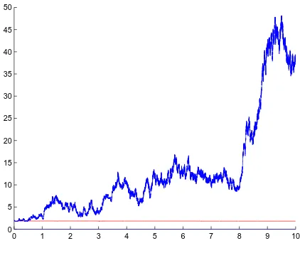
We include a numerical illustration of the pair of processesZandWof equation (1) on the zero-set of the function
f(z,w) =4z4+3z2+2wz+w3+sin(z+w)−10−sin(2).
0 1 2 3 4 5 6 7 8 9 10 0
5 10 15 20 25 30 35 40 45 50
Figure 1: The process f(Z,W) (red) and the square radial process Z Z +W W (blue) for the example above
the balls BR with any compact exhaustion of a domain D that contains an initial point where f(z0,w0) =0 for the SDE is inconsequential to the proof.
In effect, equation(1) defines a Brownian-like martingale on a Euclidean submersion of a complex manifold. The radial processk(Zt,Wt)kbehaves like the radial process of 2-dimensional Brownian motion in the ambient space stopped atRin the sense that
2E(τ) =R2 whent→ ∞and
Ek(Zt,Wt)k2=2t, whenR→ ∞.
In the manifold case the zero-setN (viewed as an embedded manifold inC2) has a natural
Rie-mannian structure and hence there is a canonical Brownian motion induced by the Kähler metric, see for instance[IW81]. In general, Brownian motion on an embedded manifold has non-zero drift coefficients and is not a martingale. However, in the special case when the embedded man-ifold has a holomorphic defining function, so there exist holomorphic local coordinates by the implicit function theorem, the intrinsic Brownian motion also turns out to be a martingale and the process defined by equation (1) is its time change. One can see this by using the implicit holomorphic local coordinates to map both processes from the ambient spaceC2onto a region of
Cwhere they are both complex martingales and hence time changed Brownian motions by Lévy’s theorem.
References
[Bas95] Richard F. Bass.Probabilistic techniques in analysis. Probability and its Applications (New York). Springer-Verlag, New York, 1995.
[IW81] Nobuyuki Ikeda and Shinzo Watanabe. Stochastic differential equations and diffusion processes, volume 24 ofNorth-Holland Mathematical Library. North-Holland Publishing Co., Amsterdam, 1981.
[Kra92] Steven G. Krantz. Function theory of several complex variables. The Wadsworth & Brooks/Cole Mathematics Series. Wadsworth & Brooks/Cole Advanced Books & Soft-ware, Pacific Grove, CA, second edition, 1992.
[Ran86] R. Michael Range. Holomorphic functions and integral representations in several complex variables, volume 108 of Graduate Texts in Mathematics. Springer-Verlag, New York, 1986.