Lead Water Pipes and Infant
Mortality at the Turn of the Twentieth
Century
Werner Troesken
a b s t r a c t
In 1897, about half of all American municipalities used lead pipes to distribute water. Employing data from Massachusetts, this paper compares infant death rates in cities that used lead water pipes to rates in cities that used nonlead pipes. In the average town in 1900, the use of lead pipes increased infant mortality by 25 to 50 percent. However, in cities using new pipes and distributing acidic water, lead pipes increased infant mortality three- to four-fold. Qualitative evidence supports the econometric results and indicates the adverse effects of lead extended beyond Massachusetts.
I. Introduction
The early-twentieth-century United States saw rapid improvements in life expectancy; this improvement was especially pronounced in the heavily ur-banized Northeast. Reductions in infant mortality account for most of the improve-ment in life expectancy (Haines 2001). The sources of the transition from high to low mortality, in the United States and elsewhere, have been the subject of extensive ac-ademic debates among demographers, economists, and historians. Typically, scholars emphasize one or more of the following three forces. For some, it was the diffusion of the germ of the theory of disease to the general population. Increased knowledge of appropriate sanitary practices led parents to adopt a variety of behaviors that helped protect infants, including breast-feeding, and boiling tap water (Mokyr
Werner Troesken is a professor of economics at the University of Pittsburgh. He is also a research associate at the National Bureau of Economic Research. This research was supported by a grant from the NIH, AG10120-09A1. Claudia Linares and Paula Canavese provided research assistance at an early stage of this project. The author thanks conference participants at the NBER, and seminar participants at Columbia University and Princeton University, especially Chris Paxson, Anne Case, and Angus Deaton. Two anonymous referees provided helpful comments as well. The usual disclaimer applies. The data used in this article can be obtained beginning January 2009 through December 2012 from Werner Troesken, Department of Economics, George Mason University, 4400 University Drive, Fairfax, VA 22030, wtroeske@gmu.edu.
[Submitted May 2003; accepted August 2007]
2000; Ewbank and Preston 1991). For others, it was investments in infrastructure re-lated to public health, such as water purification systems and sewer systems (Cutler and Miller 2004; Meeker 1972, 1976; Troesken 2004; Ferrie and Troesken, Forth-coming). For still others, it was economic growth and the associated improvements in nutrition (Fogel and Costa 1997; McKeown 1976). While these authors do not en-tirely dismiss the role of public health initiatives, they tend to assign public health a secondary role and emphasize that improvements in longevity were occurring before various public health interventions.
There is, however, little systematic evidence or consensus as to how exposure to inorganic pathogens influenced the variation in infant mortality over time and across space. Yet, there are at least three reasons to think that inorganic pollutants had a se-rious public-health repercussions during this period: the nineteenth and early twen-tieth century was characterized by rapid industrialization, limited environmental regulation and control, and poor scientific understanding of the potential harm of in-organic pathogens. In such an environment, it seems plausible that pollution would have been widespread, particularly in urban areas, and that even modest efforts to minimize exposure could have had large benefits. A central problem confronting de-mographic and economic historians concerned with measuring the effects inorganic pollution on health has been to identify and construct data sources that would allow one to accurately gauge pollution exposure over time and/or across space.
Accordingly, this paper considers a largely unappreciated source of inorganic pollu-tion: the use of lead service lines to distribute household tap water. Municipalities first installed lead service lines during the late nineteenth and early twentieth century, and in some places, the original lead pipes are still in use. In 1897, about half of all municipal-ities had water systems based exclusively, or in part, on lead service lines; the remaining cities used iron pipes or metal pipes lined with cement. The use of lead pipes was posi-tively correlated with city size. In 1900, the country’s five largest cities—New York, Chicago, Philadelphia, Saint Louis, and Boston—all used lead pipes to varying degrees. For cities with populations greater than 30,000, more than 70 percent used lead lines ex-clusively or in combination with some other type of metal (Troesken and Beeson 2003). There is widespread appreciation today about the potential dangers of even low-level lead exposure, particularly for the developing fetus and very young child. At the turn of the twentieth century, however, most scientists and medical experts were concerned about occupational lead exposure and believed water lead was a compar-atively minor public health problem (Troesken 2006, 112-13, 166-67). A handful of nineteenth- and early-twentieth-century physicians were concerned about water lead, but these researchers were routinely dismissed as cranks (see, for example, Allen 1888 and Swann 1892).
pipes and limited the amount of lead that dissolved into the water. As for corrosiveness, acidic water removed more lead from the interior of pipes than did nonacidic water. In cities using new pipes and distributing water derived from acidic sources, lead pipes had enormous effects: They increased infant mortality rates and stillbirth rates three- to four-fold. Such estimates are quite plausible when one considers just how much lead could be dissolved into household tap water as a result of lead service lines. I also pre-sent a series of quasi-natural experiments, where water lead levels were suddenly in-creased, which help to buttress the econometric findings.
II. Lead in Massachusetts Tap Water
Table 1 reports the lead levels in Massachusetts tap water in 1900 for 22 towns surveyed by the Massachusetts State Board of Health (MSBH). The ta-ble also indicates the extent to which these levels exceed the modern day EPA lead-standard of 0.0015 parts per 100,000. Health officials took two sets of samples, one for water following ordinary use, and another for water that was left standing in pipes overnight. Hyde Park and Lowell each have two separate sets of lead readings be-cause in both towns two separate water sources were used. In the median Massachu-setts town, the lead level found in water after ordinary use exceeded the modern guideline by a factor of 19; the lead level in water that stood in pipes overnight exceeded the modern guideline by a factor of 58. For three cities—Hyde Park (old well); Lowell (Cook well); and Middleborough—the average lead levels in standing water exceeded the modern guideline by factors of 202, 169, and 411, respectively. Notice that even in Cambridge and Cohasset, which had the lowest lead levels of the towns surveyed, the average lead level for water that stood in pipes overnight exceeded the modern EPA guideline by factors of four and three, respectively. If, rather than averages, one considers the observed high in each sample, lead levels exceeded the modern EPA guideline by factors as large as 750.
The lead in Massachusetts tap water came from many sources, including industrial pollution of water supplies, and the lead pipe and solder used for the interior plumb-ing of homes. Two experiments, however, suggest that service pipes (the pipes con-necting homes to street mains) were the primary source of lead in drinking water. In the first experiment, conducted by the MSBH, 18 samples of water from the Boule-vard well in Lowell were passed through iron and lead service lines. Water samples passed through an iron pipe contained one-eighth to one-third the lead found in water passed through lead pipe (MSBH 1900, 491-97). In a second and independent exper-iment conducted by two New York health officials during the 1930s, very similar findings were obtained. These officials passed water from the same source in the Catskill Mountains through lead and iron pipes. The average lead content for water that passed through the lead pipe was 0.1425 parts per liter of water; the average lead content for water passed through the iron pipe was .025, one-sixth the amount found in water from the lead pipe (Quam and Klein 1936).
Given the dangers of lead, which were not unknown at the time, one might ask why local governments and water companies chose to use lead pipes. Aside from lead, service lines were also made of plain iron or steel, galvanized iron, and cement-lined iron. Relative to these other materials, lead had two features that made it
Table 1
The Lead Content of Massachusetts Tap Water
Lead Content of Water Aftera (Content)/(EPA Level)b
Ordinary Use Standing Use Standing
Municipality Maximum Average Maximum Average Maximum Average Maximum Average
Andover 0.0171 0.108 0.0571 0.0257 11.4 7.2 38.1 17.3 Attleborough 0.1714 0.0697 0.1371 0.0905 114.3 46.5 91.4 60.3 Beverly 0.0257 0.0087 0.0314 0.0147 17.1 5.8 20.9 9.8 Bridgewater 0.0086 0.0057 0.0171 0.0143 5.7 3.8 11.4 9.5 Brookline 0.0114 0.0074 0.0286 0.0197 7.6 4.9 19.1 13.1 Cambridge 0.0086 0.0025 0.0114 0.0064 5.7 1.7 7.6 4.3 Cohasset 0.0086 0.0048 0.0086 0.0043 5.7 3.2 5.7 2.9 Dedham 0.0100 0.0082 0.0200 0.0150 6.7 5.5 13.3 10.0 Grafton 0.0229 0.0187 0.0457 0.0329 15.3 12.5 30.5 21.9 Hyde Park-new 0.0457 0.0172 0.4571 0.0329 30.5 11.6 304.7 21.9 Hyde Park-old 0.0200 0.0400 0.0457 0.3029 13.3 26.7 30.5 201.9 Lawrence 0.1371 0.0543 0.1829 0.0704 91.4 36.2 121.9 46.9 Lowell-Blvd 0.0800 0.0202 0.4000 0.0861 53.3 13.5 266.7 57.4 Lowell-Cook 0.5143 0.1608 0.4643 0.2535 342.9 107.2 309.5 169.0 Metropolitan 0.0400 0.0111 0.1371 0.0293 26.7 7.4 91.4 19.5 Middleborough 0.3429 0.1549 1.1429 0.6171 228.6 103.3 761.9 411.4 Needham 0.0171 0.0091 0.0429 0.0269 11.4 6.1 28.6 17.9 Newton 0.0714 0.0432 0.1714 0.0908 47.6 28.8 114.3 60.5 North Attleboro 0.0071 0.0049 0.0329 0.0226 4.7 3.3 21.9 15.1 Webster 0.0200 0.0100 0.0571 0.0286 13.3 6.7 38.1 19.1
The
Journal
of
Human
Wellesley 0.0152 0.0101 0.0314 0.0219 10.1 6.7 20.9 14.6 Weymouth 0.0800 0.0314 0.2286 0.1167 53.3 20.9 152.4 77.8 Mean 0.0761 0.0320 0.1705 0.0874 50.7 21.3 113.7 58.3 Median 0.0229 0.0110 0.0571 0.0290 15.3 7.3 38.1 19.3 Number of observations 22 22 22 22 22 22 22 22
a. lead content is measured as parts of lead per 100,000 units of water.
b. current EPA standards allow water to contain 0.0015 parts of lead per 100,000. The columns divide the lead levels observed in Massachusetts by this modern standard.
Source: Massachusetts State Board of Health (1900), pp. 490–93.
T
roesken
attractive to the engineers who designed public water systems: It was both malleable and durable (Committee on Service Pipes 1917, 328). Malleability reduced labor costs by making it easier to bend the service main around existing infrastructure and obstructions, and compared to iron and steel, lead was a soft and pliable metal. As for durability, the life of the typical lead service pipe was 35 years. By contrast, plain iron or steel pipe lasted 16 years; galvanized pipe 20 years; and cement lined pipe 28 years. Based solely on engineering concerns, these characteristics made lead the ideal material for service lines. As one prominent trade journal wrote, ‘‘Lead is in many respects the most satisfactory material to use for service pipes. Its pliability and its comparative freedom from corrosive action make it almost ideal from a me-chanical standpoint’’ (Engineering News, September 28, 1916, 594-96).
The two problems with using lead were its high upfront cost and its potential toxicity. In terms of upfront costs, a small iron or steel pipe that was neither galvanized nor lined was certainly cheaper than lead. But as stated above, untreated iron and steel pipes had expected life spans that were less than half that of lead pipes. Because replacing broken service mains often required digging up paved streets and working around other infra-structure such as gas and sewer mains, the costs of reduced main life overwhelmed whatever savings that were generated from reduced materials costs. As for concerns that lead service lines might poison the water they carried, most engineers believed such concerns were overblown (Engineering News, September 28, 1916, 595).
That lead worked well, from a narrow mechanical standpoint, is clear when one examines how popular lead service lines were. At the turn of the twentieth century, the use of lead service mains was widespread, particularly in large cities. This can be seen in two independent samples of cities. In 1916, the New England Water-Works As-sociation surveyed 304 cities and towns, largely in New England, and found that 95 (31 percent) of these cities used lead or lead-lined services (Committee on Service Pipes 1917, 326-30). A second and independent sample is more geographically diverse and includes 797 cities and towns observed in 1900 from all over the United States. Of these cities, 209 (26 percent) used lead or lead-lined services exclusively; 137 (17 percent) used lead or lead-lined services in conjunction with some other material type, such as galvanized iron or cement-lined iron; and 451 (57 percent) used no lead. The avail-able data suggest a strong positive correlation between lead use and city size. For cities with populations less than 8,000, 33 percent used lead service pipes. In contrast, for cit-ies with populations between 30,000 and 300,000, 72 percent used lead pipes; and for the largest cities, those with populations greater than 300,000, all but one (94 percent) used lead service pipes (Troesken and Beeson 2003).
III. Econometric Evidence
To identify the effects of lead water mains on fetal and infant death rates, variants on the following generic equation are estimated using cross-sectional data from Massachusetts for the year 1900:
yi¼a0+Fli+xib+ei;
ð1Þ
if the city employed iron, cement-lined, or some other nonleaded metal;xiis a vector
of control variables that measure such things as population, infectious disease envi-ronment, and the development of infrastructure related to public health; andeiis a
random error term.
Equation 1 is estimated using a sample of 74 Massachusetts towns. For most towns in the sample, there is information about the following (municipal-level) character-istics in the year 1900: age-specific death rates, cause-specific death rates, popula-tion, whether the town used lead water pipes or some other material such as iron, hardness of the local water supply, source of local water supply (that is, above ground or below ground), and proportion of water mains installed during the previ-ous ten years. For a small subset of the full sample (about 20 towns), there is also exact data on the amount of lead contained in household tap water from each town. Data on disease rates and water lead levels are from the Massachusetts State Board of Health, data on service pipes are from Baker (1897), and data on population and ur-ban infrastructure are from various U.S. Censusvolumes. Descriptive statistics for the sample and various subsamples are reported in Troesken (2003).
There are two concerns with the regression specified in Equation 1. First, death rates might have been measured with greater accuracy in large towns than in small ones. To address this concern, all of the observations are weighted by population us-ing the aweights algorithm in STATA. Second, it is possible that the use of lead water mains is correlated with some unidentified factor that also influences the health out-comes of young children. In which case, the estimated coefficient on the dummy for lead water lines will be biased. A priori, it is not clear whether the estimated effects of lead would be biased upward or downward. One might imagine a world where only cities that were relatively careless about health used lead service lines, in which case the coefficient on the lead-use dummy would be biased upward. Alternatively, one might imagine a world where cities that already had serious public health prob-lems avoided using lead service lines, for fear of exacerbating their probprob-lems any further. In this case, only towns with relatively low death rates would have been will-ing to risk the dangers associated with uswill-ing lead service pipes, and the coefficient on the lead dummy would be biased downward.
For the purposes of this paper, however, consider a world where the use of lead water mains was correlated with something one might call the ‘‘health conscious-ness’’ of a community. Communities that were very health conscious, and attune to the dangers of lead pipes, installed iron or cement-lined pipes, while communities that were not so health conscious installed lead service lines. Whatever its effect on the probability of using lead water lines, health consciousness also would have had an independent and significant effect on infant mortality rates. As a consequence, in-fant mortality rates would have been lower in the cities using nonlead pipes than in those using lead pipes, even if both sets of cities had chosen to use the same type of pipes.
To address the concern about omitted variable bias, five strategies are pursued. The first strategy explores the health effects of lead water pipes using age-specific death rates. Given that smaller children experienced more severe health effects from lead than older children and adults, holding everything else constant, one expects that the use of lead water pipes would have had much larger effects on, say, stillbirth rates and infant death rates (children aged 0-1) than on death rates of older children. If
the use of lead lines had been correlated with health-consciousness, one would not necessarily expect to observe this pattern. It has long been known that maternal lead exposure adversely affects fetal development and increases the risk of spontaneous abortion, stillbirth, low birth weight, and premature death among infants (for exam-ple, Bellingeret al., 1991; Hertz-Picciotto 2000; Hamilton 1919; Hu 1991; Milligan 1931; Oliver 1911; Sowers et al. 2002; Stainthorpe 1914; Swann 1889; Winder 1993).
The results of this first experiment are reported in Table 2. Aside from measures of lead exposure, the regressions include controls for city size (log of population), and overall quality of public infrastructure as proxied by typhoid rates. Regressions 1-5 use a direct measure of lead exposure: the log of the lead content in tap water from a sample of 21 Massachusetts towns. For these 21 towns, the lead content of tap water has a large and statistically significant effect on the death rates of infants and children aged one to two. For infants, an increase in lead levels by one-standard deviation would have generated an 18 percent increase in mortality rates. For children aged one to two, a one-standard-deviation increase in lead would have generated a 12 per-cent increase in mortality rates. Lead levels have no systematic effect on the mortal-ity rates of children aged two to four, or on children aged four to ten.
Regressions 5-10 identify the average effect of lead water lines on the mortality rates of young children. Notice that the sample size has more than doubled, because there are data on the use lead water lines for many more cities than there are data on the exact level of lead in tap water. The results here conform to prior expectations. The use of lead water lines had a large and statistically significant effect on the mor-tality rates of the very young, but no effect, either statistically of substantively, on the mortality rates of older children and adults. Lead water pipes increased stillbirth rates by 59 percent above the mean level observed in town’s with nonlead pipes; infant mortality rates by 39 percent; and the mortality rates of children aged one to two by 24 percent. That lead water lines had no discernible or systematic effect on the mortality rates of older children is consistent with the idea that only the smallest and least developed children were vulnerable to fatal lead poisoning related to water. The second strategy explores the correlation between lead pipes and infectious dis-ease rates. If it were a lack of health consciousness, and not lead water pipes, that drove up infant death rates in towns with lead water lines, one would expect to ob-serve a positive correlation between the use of lead water lines, and infectious dis-eases such as scarlet fever, measles, and the like. However, a positive relationship between lead use and infectious disease might also reflect the fact that exposure to unhealthy lead levels at a young age left children weak and compromised in terms of their ability to fight off infectious diseases. Hence, a positive relationship between lead use and infectious disease rates does not, by itself, prove that it was a lack of health consciousness, and not the use of lead water pipes, that caused the elevated rates of infant death in towns with lead lines. A negative coefficient, or a very small positive one, on the lead dummy would undermine the case that it was health con-sciousness, or a lack thereof, that drove up infant mortality rates in towns with lead pipes.
Table 2
Age and Vulnerability to Fatal Lead Poisoning
Effects of Lead Content Effects of Lead Pipes
(1) (2) (3) (4) (5) (7) (8) (9) (10) (11)
Dependent Variable (death rate by
age group) Still-births Infants Age 1–2 Age 2–4 Age 4–10 Still-births Infants Age 1–2 Age 2–4 Age 4–10
Log(lead content) 0.14 (4.5) 47.6*(14.8) 6.4*(3.9) 1.1 (2.0)
23.0 (2.8) — — — — —
¼1 if city used lead water lines
— — — — — 56.9*(15.9) 139.5*(33.4) 19.8*(8.9)
2.94 (6.6) 1.8 (5.8)
Log(population) 28.5*(6.5) 79.3*(21.1) 16.3*(5.6) 11.0*(2.8) 8.7*(4.0) 27.7*(8.1) 70.6*(17.0) 13.0*(4.5) 9.2*(3.4) 6.7*(2.9) Typhoid: deaths
per 100,000
0.93 (0.6) 0.29 (2.0) 0.49 (0.54)20.11 (0.27) 0.85*(0.38) 20.16 (0.6) 1.3 (1.3) 0.27 (0.32) 0.03 (0.24) 0.06 (0.21)
AdjustedR2 0.500 0.621 0.402 0.446 0.234 0.271 0.356 0.150 0.061 0.037
Number of observations
21 21 21 21 21 74 74 73 73 73
Notes: All death rates (stillbirths, infant, age 1–2, age 2–4) are reported as deaths per 100,000 persons. A constant term is included in all regressions, but is not reported. All observations have been weighted by population to control for the possibility that death rates were measured with greater accuracy in large towns than in small towns. Standard errors are reported in parentheses.
*Significant at the 5 percent level or higher (two-tailed test).
Sources: see text. Troesken
results yield no evidence of a positive correlation between the use of lead water pipes and these infectious diseases, and weak evidence of negative correlation. Troesken (2003) reports the results of these regressions in detail. A related strategy would be to look at other lead-related maladies besides infant mortality, such as suicides, crime, and eclampsia and check if they too are correlated with lead water pipes. The results of such exercises offer some support for the results reported here.1
The third strategy is to control for health consciousness directly. For example, health consciousness probably would have manifested itself in other public invest-ments such as sanitary sewers and encouraged local officials to use ground water for the public water supply—ground water was much more likely to have been germ-free than above-ground sources. By the same token, holding everything else constant, health consciousness would have also manifested itself in lower infectious disease rates. Health-conscious families and towns would have been more aggressive than those who were indifferent to health outcomes in undertaking the public and private precautions necessary to prevent the spread of infectious diseases. Accordingly, the regressions for this third empirical strategy include controls for various infectious disease rates and the presence of public health infrastructure.
Table 3 reports the results of this empirical strategy. Regressions 1-3 use death rates from two childhood infectious diseases—measles and whooping cough—and age-specific death rates for older children to capture some of the effects of health consciousness. These regressions also include death rates for older-aged children as control variables. When these direct controls are added to the regressions, the co-efficient on the lead water line dummy is reduced by half in the case of stillbirths, is reduced by about 20 percent in the case of infant deaths, and is unaffected in the case of deaths for children aged one to two. Nonetheless, the coefficient remains statisti-cally significant at high levels for all three regressions, and the estimated effect of lead water lines is still quite large. In particular, Regressions 1-3 suggest that, on av-erage, lead water lines increased stillbirth rates by 23 percent, infant mortality rates by 31 percent, and the death rate among one- to two-year olds by 25 percent. Adding controls for public health infrastructure does not alter these findings. The types of public health investments controlled for are: sanitary sewers; storm sewers; and the presence of an underground water source. See Regressions 4-6.
The fourth strategy is to employ instrumental variables. Three instruments are used to predict lead use: who financed the service pipe (the property owner or the city); the ownership history of the local water supply (always public, always private, or switched from private to public); and the number of water meters per 100 miles of water mains (a crude indicator of the complexity of the local infrastructure). As explained in Troesken (2003), lead water pipes were more likely to be used by public water companies, companies that required customers to pay for and maintain their
Table 3
Controlling for Health Consciousness Directly
Age & infectious diseases Plus public infrastructure
Variable (1) (2) (3) (4) (5) (6)
Stillbirths per 100,000 persons dependent
variable
— — dependent
variable
— —
Death rate: children 0–1 years old — dependent
variable
— — dependent
variable
—
Death rate: children 1–2 years old — — dependent
variable
— — dependent
variable Death rate: children 2–4 years old 0.127 (0.238) 2.35*(0.687) 0.369*(0.160) 0.186 (0.243) 2.37*(0.711) 0.378*(0.166) Death rate: children 4–10 years old 0.256 (0.212) 20.801 (0.609) 0.172 (0.142) 0.249 (0.215) 20.781 (0.631) 0.195*(0.147) Typhoid: deaths per 100,000 persons 0.367 (0.327) 1.95*(0.941) 0.285 (0.219) 0.401 (0.336) 1.85*(0.985) 0.289 (0.230) Measles: deaths per 100,000 persons 0.574 (0.401) 1.57 (1.15) 0.962*(0.268) 0.359 (0.423) 1.54 (1.24) 0.967*(0.289) Whooping cough: deaths per 100,000 20.130 (0.350) 0.799 (1.01) 0.388*(0.235) 20.067 (0.380) 0.406 (1.11) 0.283 (0.260)
Log(population) 8.29 (4.95) 34.3*(14.2) 6.97*(3.32) 3.44 (6.06) 30.9*(17.7) 8.16*(4.14)
¼1 if underground water source — — — 211.9 (10.2) 243.9*(30.1) 25.48 (7.01)
¼1 if city had storm sewers — — — 219.9 (19.4) 23.01 (56.8) 16.7 (13.3)
¼1 if city had some sanitary sewers — — — 220.0 (25.9) 48.7 (75.8) 15.4 (17.7)
¼1 if city had sanitary sewers — — — 224.0*(16.6) 219.6 (48.6) 20.100 (11.3)
¼1 if both sanitary and storm sewers — — — 23.8 (14.6) 21.68 (42.8) 2.72 (9.99)
¼1 if city used lead water lines 21.7*(9.68) 112.3*(27.9) 21.2*(6.49) 21.4*(10.1) 114.7*(29.7) 21.7*(6.93)
AdjustedR2 0.225 0.509 0.612 0.237 0.499 0.603
Number of observations 73 73 73 73 73 73
Notes: A constant term is included in all regressions but is not reported. All observations have been weighted by population. Standard errors are reported in parentheses. *Significant at the 5 percent level or higher (two-tailed test).
Source: see text.
T
roesken
own service pipes, and in cities with complex infrastructure (that is, those with many water meters).
As shown in Table 4, using instrumental variables weakens some results, but strengthens others. The coefficient on predicted lead use is not a significant correlate with the death rate for children aged one to two. However, the coefficient on pre-dicted lead use is a significant correlate with the stillbirth rate and the infant mortal-ity rate, and it is roughly twice the size of the coefficient on observed lead use in the comparable regressions presented in Tables 2 and 3. According to the estimates here, lead water pipes increased the infant rate by 227 to 289 deaths, or between 63 and 80 percent. As for stillbirths, lead pipes increased the stillbirth rate by 42 to 127 fetal deaths, or between 44 and 133 percent. These patterns suggest that if there were some sort of unobserved heterogeneity across towns using lead and nonlead pipes, this heterogeneity imparts a downward bias in the OLS estimates.
The fifth strategy uses interaction effects to introduce clearly exogenous variation into water lead exposure. It is well known that soft and/or highly acidic water dis-solves more lead from the interior of pipes than water supplies with hard and/or non-acidic water supplies. Similarly, more lead is dissolved from the interior of relatively new pipes than from old pipes. (See Troesken 2006, 123-40, for a review of the deter-minants of water lead levels.) I introduce clearly exogenous variation by interacting the lead dummy in Equation 1 with a measure of water softness and/or with a mea-sure of the age of local water pipes. This procedure indicates that infant mortality rates were positively correlated with water softness (and negatively correlated with the age of water pipes) in towns with lead water lines, but were uncorrelated in towns with nonlead water lines. It is difficult to argue that water softness was positively cor-related with health consciousness in cities with lead lines, but somehow uncorcor-related in cities nonlead lines. The same is true for the age of water pipes. In this way, inter-acting water softness and age of pipe measures with the lead dummy approximates a natural experiment.
The results of these interactions are reported in Table 5. In addition to the variables reported in the table, the regressions include the following control variables: the death rate for children aged two to four, the death rate for children aged four to ten, the death rate from typhoid fever, log of the town’s population, and a dummy variable indicating whether the town drew its water from an underground source. The water hardness variable here is a measure of a given water supply’s calcium and magnesium content. In towns with (without) lead pipes, the water hardness mea-sure varies from a minimum of 0.2 (0.1) to a maximum of 0.5 (6.3), with a mean of 1.56 (1.97). The econometric results suggest that hard water dissolved much less lead from the interior walls of lead pipes than did soft water, which is exactly what one would expect. Interacting the lead dummy with the measure of water hardness indi-cates that towns with hard water and lead lines had significantly lower infant and young child mortality rates than did towns with soft water and lead pipes. The co-efficient estimates further indicate that, in towns with lead pipes, increasing the water hardness level by 10 percent above the mean would have increased infant mortality rates by 2 percent.
Table 4
The Estimated Effects of Lead Pipes Using Instrumental Variables
Firstt-stage probit
Second-stage estimation
Stillbirths Infant Age1–2
¼1 if consumer pays for service line 0.433*(0.087) — — — Water meters per 100 main miles 0.003 (0.004) — — —
¼1 if water company always public omitted — — —
¼1 if water company always private 20.021 (0.070) — — —
¼1 if water company municipalized 20.337*(0.005) — — —
Other control variablesa yes yes yes yes
Predicted lead use 0.331 127.5*(30.1) 288.5*(63.9) 13.7 (18.6)
Observed lead use 0.388 — — —
Hypothesis test statisticb 14.74c — — —
Pseudo-R2 0.259 —
Adjusted-R2 — 0315 0378 0.360
Number of observations 74 74 74 74
a. The other control variables include the typhoid rate and the log of population. For the probit model, the marginal effect is reported.
b. Test that instruments (consumer pays dummy, water meters per 100 miles of mains, and ownership dummies) can be excluded from the model. c. Significant at the 0.0053 level.
A constant term is included in all regressions, but is not reported. All observations have been weighted by population. Standard errors are reported in parentheses. *Significant at the 5 percent level or higher (two-tailed test).
Sources: See text. Troesken
Table 5
Soft Water, New Pipes, and Infant Mortality
Hard water controls New water pipe controls
Variable Stillbirths Infants Age1–2 Infants A Infants B
Control variablesa yes yes yes yes yes
¼1 if city used lead water lines 40.8*(19.3) 223.7*(55.4) 40.9*(14.7) 13.5 (61.0) 2131.8*(48.3) hardness of water 22.20 (3.99) 4.97 (11.5) 2.995 (3.05) — — hardness3(lead dummy) 210.5 (10.9) 263.3*(31.3) 212.1*(8.34) — — percent of water mains newly installed — — — 280.9 (154.7) 23.80 (113.5) (percent new)3(lead dummy) — — — 450.8**(236.0) 576.0*(173.4)
¼1 if population > 60,000 — — — — 229.6 (38.4) (percent new)3(lead)3(pop > 60,000) — — — — 1367.6*(201.8)
AdjustedR2 0.230 0.547 0.524 0.532 0.755
Number of observations 64 64 64 68 68
a. The control variables include the log of population, the typhoid rate, death rate for children aged two to four, death rate for children aged four to ten, and a dummy variable equal to one if the city employed ground (as opposed to surface) water.
A constant term is included in all regressions but is not reported. All observations have been weighted by population. Standard errors are reported in parentheses. *Significant at the 5 percent level or higher (two-tailed test).
**Significant at the 6.3 percent level (two-tailed test).
Source: see text.
The
Journal
of
Human
mains had been installed in the past ten years, while in the town with the most newly installed mains, 76 percent had been installed in the past ten years. For towns with iron pipes, there is no correlation between pipe vintage and infant mortality. How-ever, in towns with lead, a strong and steep correlation emerges in at least some spec-ifications. The dummy on lead lines alone is small and insignificant, suggesting that all of the effects of lead water lines on infant mortality are to be found in cities with relatively new water lines. In the first regression (labeled Infant A), the interaction between percent new and the lead dummy is significant at only the 0.063 level (two-tailed test). However, when one allows the interaction affect to vary across large and small cities (those above and below 60,000 persons), the estimated coefficient on the interaction term (percent new3lead dummy) increases sharply and the standard errors fall. (See regression labeled Infant B.)2
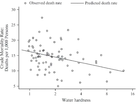
The positive correlation between soft/corrosive water supplies and premature mor-tality is not unique to turn-of-the-century Massachusetts. In a short communication to theBritish Medical Journal, Ernst E. Milligan (1931, 222-23) observed that ‘‘dur-ing the last year the infant mortality rate in an area’’ supplied ‘‘with a very lead-soluble water was 134, while that of an area in the same district in which the water had been treated to prevent lead solubility was 56.’’ Milligan noted that in the area with lead-soluble water, infantile convulsions and prematurity were prominent causes of death. In concluding his article, Milligan tried to draw a general lesson from this simple comparative exercise, writing, ‘‘In those districts with a high’’ infant mortal-ity the water ‘‘supply should be examined for the presence of lead.’’ Consider as well Figure 1, which plots city-level data on mortality against water hardness for the State of Maine in 1915. Lead water pipes were ubiquitous in Maine (Baker 1897, 34-49). There is a clear negative correlation between crude mortality (R2¼0.111) in a given town and the hardness of its water supply. The fitted trend line suggests that in towns with very soft water, the crude mortality rate was roughly 50 percent higher than in towns with the hardest water supplies. While, by themselves, these observations and correlations are merely suggestive, when juxtaposed with the results for Massachu-setts they strengthen the case that water lead was adversely affecting health.
IV. The Abortifacient Equivalent
The econometric results in Section III suggest lead water pipes had a large effect on infant and fetal mortality. The effects are so large that one needs to ask if such results are even plausible. As noted above, there is a large literature doc-umenting the connection between maternal lead exposure and poor fetal and infant health outcomes, but how can one ascertain if water lead in Massachusetts reached the threshold to pose a serious risk to the developing fetus? In particular, is there ev-idence to suggest that the lead levels observed in Massachusetts tap water (see Table 1) were sufficiently high to induce stillbirths and premature death among very young
2. There is a theoretical motivation for allowing newly installed water mains to have a different effect in large cities than in small ones. Large cities tended to have higher population densities, and therefore an additional mile of mains in a large city probably implied a much larger addition to the water system, in terms of homes newly connected, than in a small city with lower population density. See also Troesken (2004) for evidence and a more thorough discussion of this issue.
children? To address this question, an alternative measure of water lead is con-structed. Referred to here as the abortifacient equivalent, the abortifacient equivalent is a direct indicator of the toxicity of Massachusetts tap water for the very young. The assumption underlying this metric is that most of the lead exposure to the fetus and very young child occurred in utero as a result of maternal consumption of tainted drinking water.
A brief history of abortion technologies helps explain the abortifacient equivalent. During the late 1800s and early 1900s, a handful of commercial enterprises began manufacturing and marketing abortion pills made of diachylon (a lead-based plaster) in both England and the United States (Sauer 1978; Troesken 2006, 51-53). One pop-ular brand of pill was described in the medical literature only as Dr. ___’s Famous Female Pills. According to the label, these pills were ‘‘world renowned and un-equalled½sic’’ in controlling ‘‘female problems.’’ The instructions directed the pa-tient to take two pills four times a day over a two-week period. An article in the
British Medical Journalindicated that each pill contained 0.0005 grains of lead, im-plying that if a woman took the recommended daily dose of eight pills, she would have ingested 0.004 grains of lead per day (Hall 1905).
The efficacy of products like Dr. ____’s Famous Female Pills were idiosyncratic and affected some individuals more than others. Also, it is not clear how carefully the suppliers of such pills calibrated the recommended dose. The medical literature of the day indicates that more than a few women overdosed and poisoned them-selves, sometimes fatally (Wrangham 1901; Pope 1893; Branson 1899). In other cases, not enough lead was ingested and the subsequent child was born small and unhealthy. A British physician described the surviving child of one failed abortion attempt as ‘‘a puny creature’’ suffering from ‘‘consumption of the bowels’’ (Ransom 1900, 1590). However, most women apparently were able to ingest diachylon pills Figure 1
with few outward signs of lead poisoning and simultaneously terminate their preg-nancies (Hall and Ransom 1906; Sauer 1978). Other women used diachylon to dis-rupt the menstrual cycle, much like modern-day birth control pills (Pope 1893).
The abortifacient equivalent is the amount of water an individual needed to con-sume in order to have been exposed to the same amount of lead as was contained in the recommended daily dose of Dr. ____’s Famous Female Pills. LettingLequal the water-lead concentration measured as parts lead per 100,000 parts water, the aborti-facient equivalent (AE) can be expressed as:
AE¼:878=L: ð2Þ
The derivation of this equation is straightforward. First, lead levels in Massachusetts were originally reported as parts per 100,000 and these data need to be converted to grains per (U.S.) gallon such that:
y¼ ð:583Þ3ðLÞ; ð3Þ
whereyequals the lead level expressed as grains per gallon. Second, recalling that the recommended dose contained 0.004 grains of lead, the fraction of a gallon of wa-ter necessary to ingest the abortifacient-equivalent (F) is given by the following for-mula:
F¼ ð:004Þ=y
ð4Þ
Finally, because an ounce equals (1/128) of a gallon, the ounces of water that need have been consumed to reach the abortifacient-equivalent is given by:
AE¼ ðFÞ3ð128Þ: ð5Þ
Equation 2 follows by substitution.
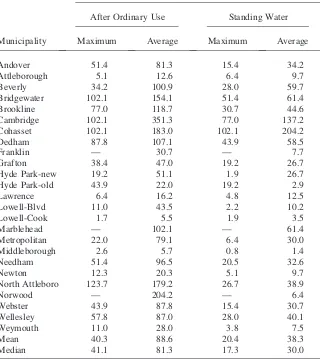
Table 6 reports the amount of lead in Massachusetts tap water in terms of the abor-tifacient equivalent. The data indicate that, in the typical town, a housewife needed to drink around 80 ounces of tap water per day to reach the abortifacient equivalent, assuming she regularly flushed her pipes before drinking tap water. If, however, the housewife did not practice flushing and regularly consumed water allowed to stand in pipes for several hours, she need only have consumed 30 to 40 ounces of tap water per day. Furthermore, this is a situation where measures of central tendency can be deceiving. Notice that in Attleborough, Lowell, and Middleborough, a house-wife need only have consumed 1 to 10 ounces of tap water daily to reach the abor-tifacient equivalent. Similarly, in Lawrence, Newton, and Weymouth, a housewife need only have consumed 6 to 28 ounces of water daily to have reached the aborti-facient equivalent.
V. Some Qualitative Evidence
A nearly ideal solution to the problem of unobserved heterogeneity would be to assemble a panel of cities and towns in Massachusetts. Although it
has not been possible to gather the data necessary to perform such an analysis, it is possible to present some qualitative evidence that comes reasonably close to a panel data analysis. In both England and Massachusetts, physicians documented numerous cases were sudden increases in water lead levels in particular towns resulted in epi-demics of water-related lead poisoning (for example, Allen 1888; Brown 1889; Ingleson 1934; Kirker 1890; Milton News, January 11, 1902, 1). Oliver (1911) Table 6
The Abortifacient Equivalent in Massachusetts Water
Ounces of Water Needed to Reach Abortifacient Equivalent
After Ordinary Use Standing Water
Municipality Maximum Average Maximum Average
Andover 51.4 81.3 15.4 34.2
Attleborough 5.1 12.6 6.4 9.7
Beverly 34.2 100.9 28.0 59.7
Bridgewater 102.1 154.1 51.4 61.4
Brookline 77.0 118.7 30.7 44.6
Cambridge 102.1 351.3 77.0 137.2
Cohasset 102.1 183.0 102.1 204.2
Dedham 87.8 107.1 43.9 58.5
Franklin — 30.7 — 7.7
Grafton 38.4 47.0 19.2 26.7
Hyde Park-new 19.2 51.1 1.9 26.7
Hyde Park-old 43.9 22.0 19.2 2.9
Lawrence 6.4 16.2 4.8 12.5
Lowell-Blvd 11.0 43.5 2.2 10.2
Lowell-Cook 1.7 5.5 1.9 3.5
Marblehead — 102.1 — 61.4
Metropolitan 22.0 79.1 6.4 30.0
Middleborough 2.6 5.7 0.8 1.4
Needham 51.4 96.5 20.5 32.6
Newton 12.3 20.3 5.1 9.7
North Attleboro 123.7 179.2 26.7 38.9
Norwood — 204.2 — 6.4
Webster 43.9 87.8 15.4 30.7
Wellesley 57.8 87.0 28.0 40.1
Weymouth 11.0 28.0 3.8 7.5
Mean 40.3 88.6 20.4 38.3
Median 41.1 81.3 17.3 30.0
describes an epidemic of stillbirths and miscarriages in a town in Yorkshire, England during the late 1890s. Upon investigation, medical officials traced the epidemic to the town’s use of lead water pipes, and once this cause was removed, the epidemic subsided and the rate of stillbirths declined. Along the same lines, Swann (1889) presents the case-histories of three women unable to conceive and/or bring a child to term while they were consuming water drawn through a lead pipe. After the lead water pipes were removed, the women eventually gave birth to healthy and robust children.
After drilling a new well for its public water supply during the 1890s—a water supply that was highly corrosive—Lowell, Massachusetts experienced one of worst outbreaks of water-related lead poisoning recorded in the modern history. Hundreds of adults and children were made sick. Eventually, the Massachusetts State Board of Health intervened and documented the most serious cases. One adult woman, who had unknowingly been suffering from lead poisoning for two years, was found to have tap water containing 1.1903 grains of lead to the gallon, or 1,357 times the modern EPA standard. She died soon after state authorities documented her case. An-other adult female was described by state authorities as a ‘‘marked invalid,’’ whose ‘‘fingers contracted on hands and hands on arms.’’ She died from a cerebral hemor-rhage shortly after her case was documented. Her tap water contained 0.2891 grains of lead to the gallon, 330 times the modern EPA standard (MSBH 1900, xxxi-xxxix). Of course, not all cases resulted in death. Much more common were nonlethal symp-toms such as ‘‘colic,’’ ‘‘constipation,’’ ‘‘loss of strength,’’ ‘‘loss of weight,’’ ‘‘emacia-tion,’’ ‘‘headache,’’and ‘‘paralysis’’ in the arms and legs. Furthermore, most cases improved once the individual stopped drinking the city’s tap water. After one woman developed paralysis in her hands and wrists, she moved from Lowell to North Billerica, where the water was much less corrosive, and made a ‘‘complete recovery.’’ Another woman had ‘‘colic and constipation’’ and eventually became so disabled she could not get out of bed. A nurse who moved into the home to take care of the bed-ridden woman soon developed similar symptoms. Analysis of tap water in the home found that it contained as much as 0.2166 grains of lead to the gallon, 247 times the modern EPA standard. Both women improved after they stopped drinking city water. In yet another case, a male who lost upper body strength and developed wrist drop, showed ‘‘marked improvement’’ after a ‘‘change of drinking water (MSBH 1900, xxxi-xxxix).’’ The board of health did not explore the effects of Lowell’s lead problem on the unborn and the very young, but given the serious symptoms that emerged among the adult pop-ulation it is not difficult to predict what was happening to the former.
Finally consider the experience of the Milford Water Company. This company provided water to two neighboring towns on the Charles River in Massachusetts, Milford, and Hopedale. Beginning in 1881, the company drew its water from three wells along the river, just north of Milford. Although this water was lead solvent, and the company used lead service pipes to connect residences to street mains, the company was not made aware of any cases of water-related lead poisoning until an investigation conducted by the Massachusetts State Board of Health in 1897. Af-ter consulting nine physicians in the Milford-Hopedale area, the board of health found that there were 16 adults suffering from mild to moderate cases of lead poison-ing, apparently of unknown origin. The board of health then analyzed the tap water in the homes of these individuals. All told, 12 homes were tested for water-lead levels,
and the findings left little doubt that lead-contaminated water was the source of the lead poisoning. In one home, the water-lead level was 14.5 parts per million (ppm), 969 times the modern EPA standard. In another home, the water-lead level was 11.6 ppm, 775 times the modern EPA standard (Baker 1897, 51; Weston 1920).
In the five years after this discovery, the Milford Water Company took several steps to reduce the lead solvency of its water supply. The company began to remove the lead service pipes and replace them with pipes made of safer materials. This, however, was a slow process because replacement was expensive. The company also abandoned the wells it had been using as the city’s water source, and began drawing water from the Charles River. Water from the river was more polluted than that from the wells, and therefore had to be filtered. The company installed a slow-sand filtration system, which not only eliminated bacterial contaminants; it also reduced the lead solvency of the river water. The introduction of these measures in 1902 and 1903 reduced the maximum ob-served water-lead levels in area homes from 1.39 ppm (627 times the modern EPA stan-dard) to 0.27 ppm (175 times the modern EPA stanstan-dard). Although 0.27 ppm is a high lead level by modern standards, it was well below the 0.5-ppm- threshold then consid-ered safe by the Massachusetts Board of Health.
After introducing a new water supply and adopting slow-sand filtration, the Milford Water Company ‘‘believed that it had done everything necessary to protect its consum-ers’’ from lead poisoning. But in 1914, a decade after these precautions had been adop-ted, ‘‘a suspicious case of illness occurred’’ in the home of an individual who employed an unusually long lead service pipe. Although the water company believed that this in-dividual had an ‘‘unusually sensitive’’ constitution, it conducted tests on the individu-al’s tap water and found unusually high lead levels. With these findings, the company began searching for an appropriate chemical treatment that would reduce water-lead levels even further. Engineers for the company found that the most effective agent was quick lime. The introduction of lime dosing in 1914 had an immediate and bene-ficial effect on water-lead levels in the area. In particular, the average water-lead level in Milford and Hopedale fell from 0.27 to 0.1 parts per million. Although the 0.1 level exceeds the modern EPA standard by a factor between six and seven, it was well below the threshold considered safe around 1915 (Weston 1920).
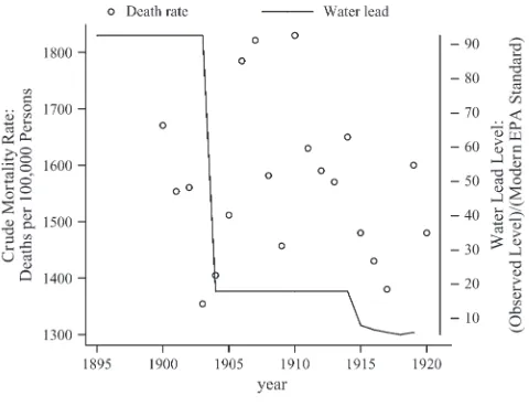
Figure 2 plots the measured (average) lead level of the Milford water supply from 1895 through 1920. There are two sharp drops in the series. The first occurs around 1902, after the introduction of water from the Charles River and the adoption of slow sand filtration; the second occurs around 1914, after the introduction of a lime-dosing system. Figure 2 also plots the crude mortality rate in Milford (measured as total deaths per 100,000 persons) between 1900 and 1920. Although it is difficult to dis-entangle the effects of lead reduction from other public health measures, it appears that the 1902 reduction in water lead was followed by a downward trend in overall mortality. Data on infant mortality, with time-consistent definitions, are not available from the U.S.Mortality Statistics, the source for Figure 2.
VI. Conclusions
source of improved infant mortality rates. In Massachusetts, the use of lead pipes to connect households to public water systems had enormous effects on infant mortality rates. In the typical Massachusetts city, lead pipes increased infant mortality rate by be-tween 25 and 50 percent. And in towns with highly acidic water, or with relatively new lead pipes, the effects were even more dramatic, with lead pipes increasing infant death rates by factors as large as three or four. These findings are robust to reasonable changes in econometric specification, and in the case of the instrumental variables estimates, are made stronger by efforts to control for unobserved heterogeneity.
Although the engineers who designed public water systems were slow to acknowl-edge the dangers of lead water lines, over time municipalities began to abandon the practice of using lead pipes, and the lead pipes that remained gradually oxidized so that less lead was taken off the interior of the pipes. Moreover, by the 1930s, the federal gov-ernment and some state govgov-ernments were actively regulating the amount lead that could be used in household plumbing systems. In Massachusetts, officials appear to have been even more aggressive and, as early as 1890, the State Board of Health was recommending that municipalities in the state abandon lead pipes. Similarly, in neigh-boring New Hampshire, public health officials began publicizing the dangers of lead service pipes during the early 1900s. According to Howard (1923, 208), lead water pipes were abandoned ‘‘by the score’’ following investigations by state health officials, which in turn resulted in significant reductions in water lead levels.
References
Allen, Alfred H. 1888. ‘‘The Sheffield Water Supply and Lead-Poisoning.’’Sanitary Record, February 15, pp. 356–57.
Figure 2
Mortality and Water Lead in Milford, Mass., 1895–20.
Baker, Moses N. 1897.The Manual of American Water-Works. New York: The Engineering News Publishing Company.
Bellinger, D., A. Leviton, and M. Rabinowitz. 1991. ‘‘Weight Gain and Maturity in Fetuses Exposed to Low Levels of Lead.’’Environmental Research54(1):151–58.
Branson, Guy J. 1899. ‘‘Lead as an Abortifacient.’’British Medical Journal, December 2, 1593.
Brown, John. 1889.Clinical and Chemical Observations on Plumbism, Due to Lead-Polluted Water; with Hints on its Prevention. Bacup, England: Tyne & Shepard Printers.
Committee on Service Pipes, New England Water Works Association. 1917. Report of Committee on Service Pipes. Presented to the Association on March 14, 1917. Reprinted in theJournal of New England Water Works Association. Volume 31. No. 3. September 1917, pp. 323–389.
Cutler, David M., and Grant Miller. 2004. ‘‘The Role of Public Health Improvements in Health Advances: The 20thCentury United States.’’ NBER working paper #10511. Ewbank, Douglas C., and Samuel H. Preston. 1990. ‘‘Personal Health Behavior and the
Decline of Infant and Child Mortality: The United States, 1900–1930.’’ InWhat We Know about Health Transitions: The Social, Cultural, and Behavioral Determinants of Health, volume 1, ed. John Caldwell, 121–45. Canberra: Health Transition Center, Australian National University.
Ferrie, Joseph P., and Werner Troesken. Forthcoming. ‘‘Water and Chicago’s Mortality Transition, 1850–1925.’’Explorations in Economic History.
Fogel, Robert W, and Dora L. Costa. 1997. ‘‘A Theory of Technophysio Evolution, with Some Implications for Forecasting Population, Health Care Costs, and Pension Costs.’’ Demography34(1):49–66.
Haines, Michael R. 2001. ‘‘The Urban Mortality Transition in the United States, 1800–1940.’’ Historical Paper, #134. National Bureau of Economic Research.
Hall, A. 1905. ‘‘The Increasing Use of Lead as an Abortifacient.’’British Medical Journal, March 18, pp. 584–6.
Hall, Arthur, and W.B. Ransom. 1906. ‘‘Plumbism from the Ingestion of Diachylon as an Abortifacient.’’British Medical Journal, February 24, pp. 428–30.
Hamilton, Alice. 1919.Women in the Lead Industries. Bulletin No. 253, U.S Department of Labor. Bureau of Labor Statistics. Washington, D.C.: Government Printing Office. Hertz-Picciotto, I. 2000. ‘‘The Evidence That Lead Increases the Risk for Spontaneous
Abortion.’’American Journal Industrial Medicine38(2):300–309.
Howard, Charles D. 1923. ‘‘Lead in Drinking Water.’’American Journal of Public Health 13(2):207–209.
Hu, Howard. 1991. ‘‘Knowledge of Diagnosis and Reproductive History among Survivors of Childhood Plumbism.’’American Journal of Public Health81(5):1070–72.
Ingleson, H. 1934.The Action of Water on Lead with Special Reference to the Supply of Drinking Water. Water Pollution Research Board. Department of Scientific and Industrial Research. Technical Paper No. 4. London: His Majesty’s Stationary Office.
Kirker, Gilbert. 1890. ‘‘The Action of Potable Waters on Lead.’’British Medical Journal, January 11, pp. 71–72.
Howard, Charles D. 1923. ‘‘Lead in Drinking Water.’’American Journal of Public Health 13(2):207–09.
Lanphear, Bruce, and K. J. Rogham. 1997. ‘‘Pathways of Lead Exposure in Urban Children.’’ Environmental Research74(1):67–73.
Maine State Board of Health. 1915.Annual Report of the State Board of Health of the State of Maine. Augusta, Me: Burleigh & Flynt, Printers.
Meeker, Edward. 1972. ‘‘The Improving Health of the United States, 1850–1915.’’ Explorations in Economic History9(3):353–73.
———. 1976. ‘‘The Social Rate of Return on Investment in Public Health, 1880–1910.’’ Journal of Economic History34(3):392–421.
McKeown, Thomas. 1976.The Modern Rise of Population. New York: Academic Press. Milligan, Ernst E. 1931. Correspondence.British Medical Journal, August 1, pp. 222–3. Mokyr, Joel. 2000.ÔWhy More Work for Mother?ÕKnowledge and Household Behavior,
1870–1945.’’Journal of Economic History60(1):1–41.
Oliver, Sir Thomas. 1911. ‘‘Lead Poisoning and the Race.’’Eugenics Review3(1):83–93. Pope, Frank M. 1893. ‘‘Two Cases of Poisoning by the Self-Administration of
Diachylon—Lead Plaster—for the Purpose of Procuring Abortion.’’British Medical Journal, July 1, pp. 9–10.
Quam, G. N., and Arthur Klein. 1936. ‘‘Lead Pipes as a Source of Lead in Drinking Water.’’ American Journal of Public Health26(4):778–80.
Ransom, W. B. ‘‘On Lead Encephalopathy and the Use of Diachylon½lead plasteras an Abortifacient.’’British Medical Journal, June 30, pp. 1590–92.
Sauer R. 1978. ‘‘Infanticide and Abortion in Nineteenth-Century Britain.’’Population Studies 32(1):81–93.
Sowers, Maryfran, Mary Jannausch, Theresa Scholl, et al. 2002. ‘‘Blood Lead Concentrations and Pregnancy Outcomes.’’Archives of Environmental Health57(4):489–95.
Stainthorpe, W. W. 1914. ‘‘Observations of 120 Cases of Lead Absorption from Drinking-Water.’’Lancet, July 25, pp. 213–15.
Swann A. 1889. ‘‘On Lead Poisoning from Service Pipes, in Relation to Sterility and Abortion.’’British Medical Journal, February 16, p. 352.
———. 1892. ‘‘A National Danger: Lead Poisoning from Service Pipes.’’Lancet, July 23, pp. 194–95.
Troesken, Werner. 2003. ‘‘Lead Water Pipes and Infant Mortality in Turn-of-the-Century Massachusetts.’’ NBER working paper.
———. 2004.Water, Race, and Disease. Cambridge: MIT Press.
———. 2006.The Great Lead Water Pipe Disaster. Cambridge: MIT Press.
Troesken, Werner, and Patty Beeson. 2003. ‘‘On the Significance of Lead Water Mains in American Cities: Some Historical Evidence.’’ InHealth and Labor Force Participation over the Life Course, ed. Dora L. Costa, 127–51. Chicago: University of Chicago Press and NBER.
U.S. Department of the Interior. Various volumes, various years.Census. Washington, D.C.: GPO.
U.S. Department of the Interior. Bureau of the Census.Mortality Statistics. Various years, 1900–1920. Washington, D.C.: GPO.
Weston, Robert S. 1920. ‘‘Lead Poisoning by Water and Its Prevention.’’Journal of the New England Water Works Association34(1):239–63.
Winder, C. 1993. ‘‘Lead, Reproduction, and Development.’’Neurotoxicology14(2):303–14. Wrangham, W. 1901. ‘‘Acute Lead Poisoning in Women Resulting from the Use of Diachylon
as an Abortifacient.’’British Medical Journal, pp. 72–74.