1. Other studies that document this phenomenon include Katz and Murphy (1992), Juhn, Murphy, and Pierce (1993), and Katz and Autor (1999).
T H E J O U R NA L O F H U M A N R E S O U R C E S • X X X I X • 3
Who Receives the College Wage
Premium?
Assessing the Labor Market Returns to
Degrees and College Transfer Patterns
Audrey Light
Wayne Strayer
A B S T R A C T
Using data from the 1979 National Longitudinal Survey of Youth, we esti-mate wage models in which college-educated workers are classified accord-ing to their degree attainment, college type, and college transfer status. The detailed taxonomy produces modest improvements in explanatory power rel-ative to standard specifications, and reveals considerable heterogeneity in the predicted wages of college-educated workers. We find that transfer stu-dents receive an “indirect” wage benefit insofar as changing colleges allows them to earn a degree. Some transfer students receive an additional “direct” wage benefit, presumably because switching schools increases their skill investment opportunities.
I. Introduction
The wage premium paid to college-educated workers in the United States rose dramatically during the 1980s. Among men aged 31–35, for example, the wage differential between high school and college graduates grew from 18 percent in 1979–81 to 41 percent in 1989–91 (Card and Lemieux 2001).1In light of this
pro-Audrey Light is an associate professor of economics at Ohio State University. Wayne Strayer is an econo-mist at Welch Consulting. We received financial support for this research from the Spencer Foundation and the American Educational Research Association, which receives funds for its AERA Grants Program from the National Center for Education Statistics, the Office of Educational Research and Improvement (U.S. Department of Education), and the National Science Foundation under NSF Grant #REC-9980573. Opinions reflect those of the authors and do not necessarily reflect those of the granting agencies. The data contained in this article may be obtained between January 2005 and December 2008 from Audrey Light, Department of Economics, Ohio State University, 410 Arps Hall, 1945 North High Street, Columbus OH 43210.
[Submitted January 2002; accepted February 2003]
found change in the U.S. wages structure, it is worth asking whether all college-educated workers receive similar labor market rewards. While data from the Current Population Surveys enable analysts to identify trends in the college premium, we must turn to detailed data on individuals’ educational experiences to learn the sources of wage variation among college-goers in a given cohort. Previous research in this vein examines the wage benefits associated with institutional quality (Loury and Garman 1995; Dale and Krueger 1998; Brewer, Eide, and Ehrenberg 1999; Hilmer 2000), two-year versus four-two-year enrollment (Grubb, 1993; Monk-Turner 1994; Kane and Rouse 1995, 1999; Leigh and Gill 1997), and college degrees (Kane and Rouse 1995, 1999; Jaeger and Page 1996; Ureta and Welch 1998).
In this study, we ask whether the wages of workers with identical college degrees vary with their college transfer patterns. Using data from the 1979 cohort of the National Longitudinal Survey of Youth, we first categorize college-educated workers according to their highest degree received. We then consider whether they attend two-year (community) college only, four-two-year college only, or a combination of two- and four-year institutions. While the latter category defines one transfer pattern, we fur-ther subdivide the “two-year only” and “four-year only” categories according to whether the individual attended multiple institutions. In contrast to crude, three-way distinctions between college graduates, college dropouts and others, we identify 11 types of college-educated individuals. By including these controls in standard wage models, we determine how predicted, post-school wages differ across these college categories, and the extent to which our detailed taxonomy reduces unexplained vari-ation in wages.
Our data reveal that transfer decisions are a prominent feature of students’ college-going experiences. More than 45 percent of associate’s degree recipients, 28 percent of bachelor’s degree recipients, and 16 percent of nondegree recipients undergo a col-lege transfer—which we define as a change in institution following no more than 11 months of nonenrollment.2One of the most striking characteristics of transfer stu-dents is that they stay in college much longer than nontransfer stustu-dents: the gap in mean enrollment duration between transfer and nontransfer students is roughly one year for bachelor’s degree recipients and two years for nondegree recipients. Moreover, transfer students often have higher levels of measured ability than non-transfer students and live in states with more colleges. We control for these and other factors in our wage models in order to isolate the effects of transferring from the con-founding effects of related observables.
We find that predicted wages for transfer students are at least as large as those for observationally equivalent nontransfer students. Transfers increase wages indirectly by facilitating graduation, but they also can have an additional, direct effect on wages. We predict a direct wage premium of 6–7 percent for bachelor’s degree recipients who transfer between four-year colleges and for students who attend multiple two-year colleges without earning a degree. In general, we expect students to benefit from transferring if they succeed in finding better environments for skill acquisition. Four-year college students are particularly likely to engage in college “matching,” given the
wide range of educational opportunities available to them. If two-year students out-side a degree track are primarily interested in job training, then they, too, are likely to switch colleges in order to gain additional skills. The wage premium of 6–7 percent among these groups can be viewed as the average “return” to successful college matching.
Our focus on transfer patterns as a dimension of the college-going experience dis-tinguishes our research from most of the “returns to schooling” literature. We are aware of only two other studies that estimate wage models after accounting for work-ers’ college transfer status. Kane and Rouse (1995) identify separate parameters for workers with bachelor’s and associate’s degrees, as well as for nondegree recipients who attend two-year college, four-year college, or both. Thus, they isolate the mean wages of a particular type of transfer student: college dropouts who make a two- to four-year transition. Hilmer (2000) estimates separate wage models for bachelor’s degree recipients who attend a single four-year college, multiple four-year colleges, and both two- and four-year colleges, but he assesses inter-group differences in the returns to college quality rather than predicted wages. A number of analysts model the decision to transfer colleges (Velez and Javalgi 1987; Lee and Frank 1990; Jones and Lee 1992; Kearney, Townsend, and Kearney 1995; Hilmer 1997) without examining labor market outcomes. Rouse (1995) looks at two- to four-year transfer students’ eventual educational attainment, while Hilmer (1997) considers the quality of their post-transfer institutions. This body of research has revealed a great deal about col-lege transfer behavior, but we believe ours is the first study to offer comprehensive evidence on the wages associated with various transfer patterns.
II. Why Do College Students Transfer?
Our primary goal is to identify the wage gains associated with college transfers. In our empirical analysis, we specify flexible wage models that allow the transfer premium or penalty to vary across transfer types. In this section, we consider the avenues through which transfer-wage relationships might arise.
Information-based models of college decisions (Comay, Melnik, and Pollatschek 1973; Manski 1989; Altonji 1993) provide a general framework for evaluating college transfers. These models take the view that college entry is an experiment—or, stated differently, that college investment decisions occur in a dynamic environment and may periodically be revised. We argue that students may decide to change schools after reassessing the costs and benefits of their investment options. On the benefit side of the equation, students may learn about their own aptitudes and the academic rigors of their current (or prospective) colleges and decide that they would be better matched at a different institution.3They may also transfer in order to alter their course of study, perhaps after updating their beliefs about the labor market payoffs associated with different types of skills. On the cost side, students may transfer to lower their tuition
3. Light and Strayer (2000) find that the match between measured student ability and college quality is an important determinant of college completion rates. Loury and Garman (1995) consider the link between student-college matches and subsequent wages. Neither study considers transfer decisions explicitly. The Journal of Human Resources
bill or living expenses, or to improve their part-time employment prospects or finan-cial aid package. Of course, transferring colleges can also increase college costs, especially when it entails longer enrollment durations. Just as early-career job mobil-ity is seen as a search for productive employment relationships (Jovanovic 1979a, 1979b; Topel and Ward 1992), we view college transfers as a process of matching individuals and colleges, where the match depends on both the benefits and costs associated with each educational opportunity.
If students switch colleges in pursuit of a better match, what are the implications for post-college wages? Individual students can experience bad luck and discover ex post that their transfer decisions failed to improve their match. On average, however, the transfer process should increase the quality of student-college matches. As long as students focus on investment-related college attributes in attempting to improve match quality, transfers will, in turn, enhance the probability that a degree is obtained and increase future wages. Therefore, transfers will have an indirecteffect on future wages via their effect on degree attainment. Consider students who begin their course-work at a two-year college and later transfer to a four-year college. If they succeed in improving their match via the upward transfer, they stand a good chance of receiving a bachelor’s degree. If they make a “bad” transfer (and prove unable to handle the aca-demic rigors of a four-year college, for example) they are unlikely to receive a bach-elor’s degree. By holding transfer pattern constant and comparing predicted wages of degree and nondegree recipients, we can assess the indirectwage benefit of improv-ing one’s match—that is, the effect that operates via degree recipiency.
Transfers will have a separate, directeffect on wages if they improve opportunities for skill investment beyond what is reflected in the receipt of a degree. For example, high-ability students who initially enroll at “run of the mill” colleges may transfer to more selective, academically challenging institutions, or to schools with specialized programs that match their academic interests. If these transfers lead to improved train-ing that is subsequently rewarded in the labor market, they have a direct effect on wages. We can assess this effect by holding degree constant and comparing predicted wages of transfer and nontransfer students.4
There are at least two reasons why the data might fail to reveal a positive relation-ship between wages and transfers. First, transfer decisions may be driven by factors unrelated to matching or, more accurately, unrelated to matching on investment-related criteria. The notion that early-career job mobility is an ongoing matching process has been contrasted with the alternative hypothesis that workers are inherently either movers or stayers. Similarly, the population of college switchers could be dom-inated by movers—for example, students who are reluctant to commit to a particular academic program or institution. Students also may choose to transfer to alter their proximity to family or friends, or upon learning more about the social atmospheres of alternative colleges. These students are searching for “better” colleges, but along dimensions that are unlikely to affect their marketable skills (except insofar as stu-dents who enjoy their environment are likely to perform better in the classroom).
Second, even if students’ transfer decisions improve their investment opportunities and increase their future wages on average, we might fail to identify these intra-per-sonal wage gains in the data. Suppose students with high ability, college-oriented peers, and/or attentive high school guidance counselors make better initial college-related choices than other students and, as a result, are less likely to transfer. If these same characteristics increase wages and we do not control for them in our wage model, it will appear that immobility “causes” higher wages. More generally, we will fail to identify the causal effects of transfers on wages if we do not control for factors that influence the transfer decision and also have independent effects on wages. We defer to Section V additional discussion of this endogeneity problem.
Although the decision-making we describe broadly applies to all college stu-dents, we might see systematic differences across segments of the college-going population. In particular, students who attend two-year colleges can be placed into three distinct categories (Kane and Rouse 1999): (1) those who begin their course-work at a two-year college with the hope of transferring to a four-year college; (2) those who seek job-related training; and (3) those who intend to earn a vocational degree. When students in the first category make an upward transfer they are, by definition, seeking a better match. When students in the second category switch col-leges to obtain additional job training, they may face relatively little ex ante uncer-tainty about the opportunities available to them; they may even enroll in each training course at the behest of an employer. We expect relatively few students in the third category to seek better matches among two-year institutions. Whereas stu-dents attending four-year institutions have numerous dimensions on which to match (the quality and variety of academic programs, the quality of the student body, tuition costs) vocational students choose colleges on the basis of a smaller set of cri-teria, such as proximity to home or work (Kearny, Townsend, and Kearney 1995; Kane and Rouse 1999). With these differences in mind, we allow estimated transfer effects to vary across transition type (two-year to two-year, four-year to four-year, and two-year to four-year).
III. Data
A. Samples
We use data from the 1979 National Longitudinal Survey of Youth (NLSY79), which tracks the educational and labor market experiences of 12,686 men and women born in 1957–64. Respondents are interviewed annually from 1979 to 1994 and biennially thereafter; we use data for 1979–96.
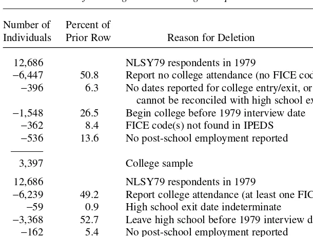
The criteria we use to select our samples are summarized in Table 1. To identify college-goers, we first eliminate 6,447 respondents who report no college attendance. NLSY79 respondents are repeatedly asked to report the entry and exit dates (month and year) and names of the last few colleges attended; college names are coded using Federal Interagency Committee on Education (FICE) codes. Anyone for whom no FICE code appears during any interview year is deemed not to have attended college. We then eliminate 396 respondents whose college entry and exit dates are missing or at odds with reported high school graduation dates. Next, we eliminate 1,548 respon-The Journal of Human Resources
dents who attend college prior to their 1979 interview date. By imposing an analogous selection rule for our noncollege sample, we ensure that all respondents come from similar high school cohorts and that no early-career employment experiences precede the observation period. We also eliminate 362 respondents whose FICE codes do not appear in the Integrated Postsecondary Data System (IPEDS), which contains detailed information on virtually all postsecondary institutions in the U.S.5 This criterion ensures that all college spells we track are “legitimate,” and also allows us to use IPEDS to identify characteristics of each college, including whether it is a two-year or four-year institution. After eliminating 536 respondents for whom no post-school employment is reported, we are left with a sample of 3,397 college-goers.
The criteria we use to select a sample of noncollege-educated workers are summa-rized in the bottom panel of Table 1. Beginning with the 6,447 NLSY79 respondents for whom no FICE codes are available, we simply eliminate 59 individuals whose date of high school exit is unknown, 3,368 individuals who leave high school prior to their 1979 interview date, and another 162 individuals who report no post-school employment experiences. These criteria yield a sample of 2,858 noncollege-goers. We combined them with our college-goers to obtain a sample size of 6,255 individu-als with which to estimate the wage models.
5. IPEDS data are collected by the National Center for Education Statistics of the U.S. Department of Education.
Table 1
Selection Criteria for College and Noncollege Samples
Number of Percent of
Individuals Prior Row Reason for Deletion
12,686 NLSY79 respondents in 1979
−6,447 50.8 Report no college attendance (no FICE code)
−396 6.3 No dates reported for college entry/exit, or dates cannot be reconciled with high school exit
−1,548 26.5 Begin college before 1979 interview date
−362 8.4 FICE code(s) not found in IPEDS
−536 13.6 No post-school employment reported
———
3,397 College sample
12,686 NLSY79 respondents in 1979
−6,239 49.2 Report college attendance (at least one FICE code)
−59 0.9 High school exit date indeterminate
−3,368 52.7 Leave high school before 1979 interview date
−162 5.4 No post-school employment reported
———
B. Defining College Transfers
In characterizing the college experiences of the 3,397 college-goers in our sample, we confine our attention to the sequence of colleges attended prior to (but possibly cul-minating in) the receipt of a bachelor’s degree. Individuals who subsequently earn a graduate degree are identified as such in our wage models, but our goal is to classify individuals in terms of their undergraduate college enrollment. We first determine whether the highest undergraduate degree received is a bachelor’s or an associate’s. College-goers who receive neither of these degrees fall into the “some college, no degree” category.
Next, we define a dummy variable to indicate whether each respondent transfers between colleges. To do so, we must consider what is meant by a transfer. We could use the broadest definition possible and classify as a transfer student anyone who attends multiple colleges during the observation period. At the other extreme, we could consider the definition typically used by colleges: transfer students are the sub-set of switchers who receive credit for courses completed at a previous institution (McCormick and Carroll 1997). We cannot directly apply the latter definition because we do not know whether college switchers are granted transfer credit. We opt not to use the former definition because, in our data, students leave school for as long as 10 years before reenrolling. While Leigh and Gill (1997) find that individuals who earn an associate’s degree after a sizeable enrollment interruption receive a higher wage premium than do students who receive their schooling continuously, Light (1995) finds that, in general, the return to “interrupted” schooling is substantially lower than the return to continuous schooling.
To avoid confounding the effects of enrollment interruptions with the effects of transferring, we follow individuals from their first college entry to the start of their first nonenrollment spell lasting 12 months or more; anyone attending multiple col-leges within that interval is defined as a transfer student.6We also experiment with three alternative definitions in which we classify as transfers: (1) all college switches; (2) all college switches prior to age 26; and (3) all college switches after dropping from the sample individuals whose nonenrollment spells account for more than 20 percent of the elapsed time from first college entry to last college exit. Although we do not report results based on these alternative definitions, in Sections IV and V we indicate the extent to which our findings are sensitive to the definition used.
C. Variables
Most estimates of the returns to schooling are based on cross-sectional data, but we use multiple wages reported by workers after receiving their highest degree. Our regression sample contains 48,266 wage observations for 6,255 workers.7 If we instead drew a cross-section based on elapsed time since school exit, we would have
6. Students who return to the same college after a nonenrollment spell are not counted as transfer students. Moreover, college spells that are “enclosed” in other spells are not counted; this excludes from the transfer category students who take a summer course at a college other than their primary institution.
7. We use wages reported through 1996, or until the last interview date of respondents who drop out of the survey. Each respondent contributes, at most, one wage observation per survey year.
The Journal of Human Resources
virtually no variation in work experience. A cross-section drawn from a particular inter-view year would induce a strong correlation between schooling attainment and experi-ence. We avoid both problems by using multiple wages for each respondent. Although no sample member is observed beyond age 40, we are able to maximize the available variation in work experience and estimate a conventional, life-cycle wage profile.
Summary statistics for the variables used in our wage models appear in Table 2. The dependent variable is the natural logarithm of the average, hourly wage divided by the implicit price deflator for gross domestic product. The covariates can be grouped into three categories: schooling measures, nonschooling baseline variables, and an additional set of variables (ability, college enrollment duration, and so forth) that prove to be related to college enrollment patterns. The schooling measures include 11 dummy variables that classify college-educated workers according to degree (none, associate’s, bachelor’s), transfer status (yes or no), and college type (two-year only, four-year only, or both). We identify noncollege-goers’ schooling attainment with three additional dummy variables indicating whether they have a high school degree (the omitted schooling group), drop out of high school after complet-ing Grade 8, or drop out at an earlier grade level. We also control for whether work-ers hold a graduate degree; everyone in this category is identified as a bachelor’s degree recipient as well.
Our additional baseline covariates are dummy variables indicating whether the respondent is male, black, and Hispanic, calendar year dummies, and continuous measures of actual work experience. We define experience as the cumulative number of hours worked from the twentieth birthday to the date the wage is earned, divided by 2,000 for conversion to full-time, full-year equivalents.8Our goal is to control for all post-school work experience, plus in-school experience from age 20 onward. Because some individuals leave school prior to their twentieth birthday, we also con-trol for cumulative hours worked (divided by 2,000) from school exit until the twen-tieth birthday; this variable equals zero for anyone leaving school after age 20. Failure to control for in-school experience causes its wage-enhancing effects to be absorbed by the college variables (Light 2001). Transfer students gain relatively more work experience than nontransfer students, so the omitted variable bias would potentially be greater for our key covariates.9
As we demonstrate in the next section, transfer and nontransfer students tend to dif-fer in their measured ability, the number of colleges in their state, and the cumulative duration of their undergraduate enrollment. We control for ability using respondents’ percentile scores on the Armed Forces Qualifying Test (AFQT).10From IPEDS, we
8. We construct this measure from the weekly hours worked variables in the NLSY79 Work History file. These variables account for within- and between-job gaps and dual job-holding, and are available for every week from 1978 forward. We choose to initialize work experience at a uniform date for each respondent (the twentieth birthday) rather than at an endogenously determined date such as the start of the first job. Any date that depends on high school exit or first jobs would occur before 1978 for some respondents, thus causing their measured experience to be left-censored.
The Journal of Human Resources
754
Table 2
Summary Statistics for Selected Variables Used in Wage Models
Mean (Standard
Variable Deviation)
Dependent variable
Natural logarithm of average hourly wagea 2.07
(0.61) Schooling and baseline covariates
1 if received no high school diploma, highest grade≤8 0.03
1 if received no high school diploma, highest grade>8 0.13
1 if attended some college, received no degree 0.24
1 if received associate’s degree 0.05
1 if received bachelor’s degree or higher 0.15
1 if received master’s, doctorate or professional degree 0.02
1 if male 0.56
1 if black 0.26
1 if Hispanic 0.18
Cumulative years of work experience since age 20b 5.16
(4.01)
Cumulative years of work experience before age 20c 0.56
(0.79) Additional covariates
Percentile score on Armed Forces Qualifying Test (AFQT) 36.84
(26.67)
Number of public, two-year colleges in state 2.75
per 100,000 residents age 18–26d
(0.98)
Number of public, four-year colleges in state 1.52
per 100,000 residents age 18–26d (0.82)
Cumulative duration of enrollment in two-year 0.46
colleges (total months divided by 12) (1.19)
Cumulative duration of enrollment in four-year colleges 0.83
(total months divided by 12) (1.73)
Number of person-year observations 48,266
Number of individuals 6,255
a. Divided by implicit price deflator for gross domestic product; base year is 1992.
b. Cumulative hours worked from week of twentieth birthday to week wage is earned, divided by 2,000. c. Cumulative hours worked from week of school exit to week of twentieth birthday, divided by 2,000; zero if respondent leaves school after twentieth birthday.
obtain the number of two- and four-year colleges in each student’s state in the year he/she finished high school (if a noncollege-goer) or began the first college spell (if a college-goer). We divide these figures by the number of 18–26-year-old residents in the same state-year cell. These variables are intended to measure the number of in-state alternatives facing respondents as they make their college matching decisions; if we omit the denominator or control for total enrollment (number of seats, rather than number of schools) as a percent of the college-aged population, we obtain virtually identical results. Using self-reported entry and exit dates (month and year) of each college attended prior to receiving a bachelor’s degree, we also measure the cumula-tive number of months each college-goer spends in two-year colleges and four-year colleges. The enrollment duration variables equal zero for individuals who do not attend college.
IV. Degree Recipiency and College Transfer Patterns
Table 3 shows how the 3,397 college-goers in our sample are classi-fied in terms of highest degrees received and college enrollment patterns. The bottom row shows that students in the “some college, no degree” category are the least likely to transfer. Just over 16 percent of these students transfer, compared to 45 percent of students who eventually receive associate’s degrees and 28 percent of bachelor’s degree recipients.11The “some college” students who transfer are distributed quite evenly among two-year to two-year transitions (5.7 percent of the sample), four-year to four-year transitions (5 percent), and transitions from two-year to four-year institu-tions (5.4 percent). Associate’s degree recipients are much more likely to transfer from two-year to four-year colleges (34.2 percent) than among two-year colleges (11.2 percent). Among bachelor’s degree recipients, 15.1 percent start their postsec-ondary schooling at a two-year college before transferring, while the remaining 13.1 percent switch among four-year colleges.
Table 3 also allows us to see how degree recipiency varies by college enrollment pattern. Among students who attend a single two-year college, 18.7 percent (244 out of 1,304) ultimately receive an associate’s degree. While this number is close to the 16 percent graduation rate reported in Kane and Rouse (1999), it masks the fact that the relatively few students who attend multiple two-year colleges are considerably
morelikely to receive a degree: their graduation rate is 32 percent (50 out of 156). Among students who attend only four-year institutions, the graduation rate does not vary significantly by transfer status; 61 percent end up with a bachelor’s degree regardless of whether or not they attend multiple colleges. Only 24 percent (100 out of 417) of students who attend both two- and four-year colleges end up withouta col-lege degree, although individuals in this category are less likely to earn bachelor’s degrees than are students in the “four-year only” category. In summary, Table 3
The Journal of Human Resources
756
Table 3
Distributions of College Enrollment Patterns by Highest Degree Received
Highest Degree Received
Some College,
College enrollment pattern no Degree Associate’s Degree Bachelor’s Degreea All Degrees
Number Percent Number Percent Number Percent Number Percent
Two-year college
No transfer 1060 56.9 244 54.6 1304 38.4
Transfer 106 5.7 50 11.2 156 4.6
—— —— —— —— —— ——
All two-year only patterns 1166 62.6 294 65.8 1460 43.0
Four-year college
No transfer 503 27.0 781 71.8 1284 37.8
Transfer 93 5.0 143 13.1 236 6.9
—— —— —— —— —— ——
All four-year only patterns 596 32.0 924 84.9 1520 44.7
Two-year and four-year college
Transfer 100 5.4 153 34.2 164 15.1 417 12.3
All college-goers 1,862 100.0 447 100.0 1,088 100.0 3,397 100.0
All transfers 299 16.1 203 45.4 307 28.2 809 23.8
reveals that (a) transfers are surprisingly prevalent, (b) transitions between two- and four-year colleges represent only half of all transfers, and (c) transfer decisions do not appear to detract from the probability of degree attainment.
In Table 4, we ask how transfer and nontransfer students compare in other dimen-sions of their college-related experiences. For each of the 11 college “types,” we com-pute the mean AFQT score, number of in-state colleges as a percent of the college-aged population, and cumulative enrollment duration. Table 4 reveals that transfer students often have higher mean AFQT scores (measured ability) than their nontransfer counterparts. This is especially true in the “some college, no degree” cat-egory: students who attend a single two-year college have a mean AFQT score of 38.7, while the mean for students who attend multiple two-year colleges is eight per-centile points higher. An even larger gap is seen among transfer and nontransfer stu-dents who attend four-year colleges without earning degrees, while the mean AFQT score for students who combine two- and four-year colleges (48.4) lies between the means for the other two transfer categories. Among associate’s and bachelor’s degree holders, the transfer-nontransfer gap in mean AFQT scores is much smaller and not always statistically significant. Not surprisingly, associate’s degree recipients who attend four-year colleges have the highest mean AFQT score (51.4) in their degree category, while bachelor’s degree recipients who attend two-year colleges have the lowest mean score (60.2) in their category.
Table 4 also reveals whether observed transfers are linked to the number of colleges available in the market, which we define as the state of residence. By drawing once again on the job mobility literature, we predict that students who face a relatively dense distribution of potential colleges are able to “match”—that is, switch colleges— at a lower cost than students who face a sparse distribution. The availability of two-year colleges differs dramatically across states (Rouse 1998), so a more specific prediction is that transitions among (and from) two-year colleges are concentrated in certain states. If states with a high density of colleges differ systematically from other states in their wage structure, our estimated transfer effects could simply reflect the effects of living and working in college-rich states. Table 4 contains mixed evidence on the correlation between transfers and numbers of colleges. Among “some college” students, those who transfer between two-year colleges live in states that average 2.22 two-year colleges per 100,000 college-aged residents, which is fewer than the average ratio of 2.46 for their nontransfer counterparts. The mean number of four-year col-leges is roughly the same (about 1.75 per 100,000 college-aged residents) among transfer and nontransfer students who attend four-year colleges without receiving a degree. However, associate’s degree recipients who attend multiple two-year colleges live in states with significantly more two-year colleges (2.72 per 100,000) than do their nontransfer counterparts (2.31); a similar pattern is seen for four-year colleges in the bachelor’s degree sample.
The Journal of Human Resources
758
Table 4
Sample Means and Standard Deviations for Selected Characteristics by Highest Degree Received and College Enrollment Pattern
Some College, no Degree Associate’s Degree Bachelor’s Degreea
Two-year Four-year Two- and Two-year Two- and Four-year Two- and
Covariate only only four-year only four-year only four-year
Nontransfer students
Percentile score on AFQT 38.70 46.39 46.61 67.76
(0.28) (0.42) (0.63) (0.33)
Number of two-year colleges 2.46 2.08 2.31 2.17
in state per 100,000 residents (0.01) (0.02) (0.03) (0.01)
Number of four-year colleges 1.33 1.75 1.40 1.59
in state per 100,000 residents (0.01) (0.02) (0.02) (0.01)
Cumulative years enrolled in 1.54 2.34
two-year colleges (0.02) (0.04)
Cumulative year enrolled in 1.84 4.12
four-year colleges (0.03) (0.02)
Light and Strayer
759
(1.12) (1.06) (1.18) (1.49) (0.88) (0.78) (0.77) Number of two-year colleges 2.22b 1.98b 2.37 2.72b 2.25 2.28b 2.33
in state per 100,000 residents (0.03) (0.04) (0.04) (0.08) (0.03) (0.04) (0.03) Number of four-year colleges 1.13b 1.74 1.41 1.29b 1.74 1.78b 1.30
in state per 100,000 residents (0.02) (0.05) (0.03) (0.04) (0.04) (0.04) (0.02)
Cumulative years enrolled 3.17b 1.74 3.37b 2.70 2.08
in two-year colleges (0.10) (0.09) (0.06) (0.06) (0.04)
Cumulative year enrolled 3.92b 2.17 1.85 5.18b 3.52
in four-year colleges (0.11) (0.10) (0.08) (0.06) (0.03)
Number of observations 550 461 492 210 786 847 957
a. Includes individuals who subsequently earn a master’s, doctorate, or professional degree.
enrollment duration of transfer students is about one year (or 25 percent) longer than that of nontransfer students. Among associate’s degree recipients, students who attend multiple two-year colleges stay in school an average of one year (or 50 percent) longer than students who attend a single school. Associate’s degree recipients who attend both two- and four-year colleges tend to be enrolled for more than twice as long as are nontransfer students.
On average, transfer students have higher measured ability and stay in college longer than their counterparts who attend a single college. In many instances, they also live in states with more of the type of college (two-year or four-year) to which they end up transferring. The models presented in the next section are designed to iso-late the wage effects of switching colleges from the effects of ability, college avail-ability, and longer enrollment duration.12
V. Wage Models
A. Labor Market Returns to Degrees and College Transfer Patterns
To assess the wage effects of workers’ college degrees and transfer patterns, we esti-mate variants of the following wage model:
K
( )1 Wit DROP8i DROP11i
冱
( D γ D T) X εk
k ik k ik i it it
0 1 2
1 $
=α +α +α + β + +δ +
= l
where the dependent variable is the log of the average hourly wage earned by worker
iat time t, Xitrepresents the nonschooling-related controls described in Section III,
and εitrepresents unobserved factors. The remaining variables in Equation 1 identify
workers’ schooling levels. Workers who do not attend college are classified as high school dropouts with no more than eight years of school (DROP8i), high school
dropouts with more than eight years of school (DROP11i), or high school graduates
(the omitted group). College-educated workers are classified by dummy variables identifying their degree and/or college type(s) (Dik) and transfer status (Ti).
In our first specification, we ignore college transfer status (that is, impose the con-straint γk = 0) and define three Dik to identify college-goers as “some college, no
degree,” associate’s degree recipients, or bachelor’s degree recipients. In the second specification, we expand Dikto seven elements by dividing each degree category
according to whether the individual attended two-year college only, four-year college only, or both. In Specification 3, we interact the same seven Dikwith Tito distinguish
between transfer and nontransfer students. This gives us the 11 college categories sum-marized in Tables 3–4, although it is important to recognize that γkin Equation 1
iden-tifies marginaleffects of each transfer category. We cannot separately identify βkand γk
for students who attend both two- and four-year colleges because Tialways equals one.
12. We also investigated differences in college quality—an inherently difficult characteristic to measure, especially when we need a metric that applies to both two-year and four-year colleges. We find positive cor-relations between transfers and college expenditures and, among four-year students, a weak, positive corre-lation between transfers and median SAT scores of incoming freshmen. However, none of these measures have any effect on our estimated coefficients of interest. Hilmer (1997, 2000) provides detailed evidence on the relationship between transfers and college quality.
The Journal of Human Resources
As described in Section III, the sample used to estimate variants of Model 1 con-tains 48,266 wage observations for 6,255 workers. We use ordinary least squares (OLS) to estimate the models, and we report robust standard errors that account for nonindependence of observations within person-specific clusters.
An important strand of the “returns to schooling” literature uses instrumental vari-ables estimation and other methods to account for the endogeneity of schooling attain-ment (see Card 1999 for a review). In our application, the dummy variables Dikand
Ti are endogenous if different types of college students are inherently different in
terms of unmeasured ability and other factors contained in εit. Moreover, transitory,
unobserved factors that drive transfer decisions (such as expectations about the labor market payoffs associated with a new course of study) also may affect post-college wages. However, the extension of instrumental variables methods to models that replace highest grade completed with indicators of degree recipiency and college enrollment patterns is far from trivial, for the “first stage” entails a sequence of multi-nomial, discrete choices. Rather than attempt to estimate a very complicated choice model jointly with the wage model, we follow Kane and Rouse (1995) in relying on ability measures (AFQT scores) to control for factors that drive students’ college-going decisions; we also control for enrollment duration and in-state college avail-ability. If Dikand Ticontinue to be correlated with εit, then we fail to identify causal
effects of various college patterns on subsequent wages.
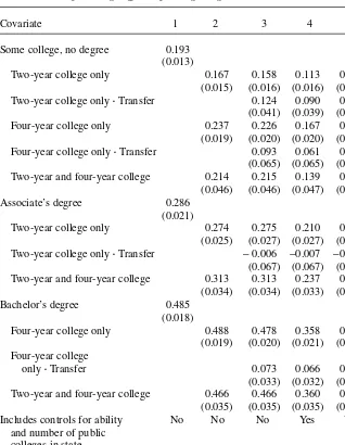
Estimates for the first two specifications are presented in Columns 1–2 of Table 5.13 These are comparable to the specifications reported in Kane and Rouse (1995), Jaeger and Page (1996), Leigh and Gill (1997), and Ureta and Welch (1998), and are intended to serve as benchmarks. The Column 1 estimates indicate that, all else equal, individuals who attend college without receiving a degree are predicted to earn 21 percent more than high school graduates (exp(.193)-1), associate’s degree recipients are predicted to earn 33 percent more, and bachelor’s degree recipients are predicted to earn 62 percent more. When we sort individuals in each degree category according to whether they attend two-year colleges, four-year colleges, or both (Column 2), it becomes evident that considerable heterogeneity exists within some of these groups. Predicted log-wages of nondegree holders who attend four-year college(s) exceed those of their counterpart who attend two-year college(s) by 0.07 (0.237−0.167), while the predicted log-wages of individuals who attend two- and four-year colleges lie in between. Associate’s degree holders are predicted to receive a 0.04 log-wage premium if they advance to a four-year college, while bachelor’s degree recipients have virtually the same predicted wage regardless of whether they attend a two-year institution.
In Columns 3–5, we add transfer interactions to distinguish among the 11 cate-gories of college-educated workers described in preceding sections. In Column 4 we add AFQT scores and measures of college availability (the number of public two- and four-year colleges in the state per 100,000 college-aged residents) to our set of con-trols, and in Column 5 we add enrollment duration as well. Specification 5 is our pre-ferred model, so we use it to draw detailed inferences about the direct and indirect wage effects of transferring. We then consider how these findings are affected when
The Journal of Human Resources
762
Table 5
OLS Estimates of the Wage Effects of College Degrees and Enrollment Patterns
Covariate 1 2 3 4 5
Some college, no degree 0.193
(0.013)
Two-year college only 0.167 0.158 0.113 0.088
(0.015) (0.016) (0.016) (0.019)
Two-year college only •Transfer 0.124 0.090 0.070
(0.041) (0.039) (0.040)
Four-year college only 0.237 0.226 0.167 0.105
(0.019) (0.020) (0.020) (0.027)
Four-year college only •Transfer 0.093 0.061 0.022
(0.065) (0.065) (0.064)
Two-year and four-year college 0.214 0.215 0.139 0.047
(0.046) (0.046) (0.047) (0.052)
Associate’s degree 0.286
(0.021)
Two-year college only 0.274 0.275 0.210 0.173
(0.025) (0.027) (0.027) (0.031)
Two-year college only •Transfer −0.006 −0.007 −0.028
(0.067) (0.067) (0.067)
Two-year and four-year college 0.313 0.313 0.237 0.144
(0.034) (0.034) (0.033) (0.042)
Bachelor’s degree 0.485
(0.018)
Four-year college only 0.488 0.478 0.358 0.237
(0.019) (0.020) (0.021) (0.042) Four-year college
only •Transfer 0.073 0.066 0.061
(0.033) (0.032) (0.032)
Two-year and four-year college 0.466 0.466 0.360 0.210
(0.035) (0.035) (0.035) (0.051)
Includes controls for ability No No No Yes Yes
and number of public colleges in state
Includes controls for No No No No Yes
enrollment duration
we fail to account for worker ability, college availability, and enrollment duration (Columns 3–4).
Focusing first on students who attend onlytwo-year colleges, the Column 5 esti-mates reveal the following. First, among workers who attend a single two-year col-lege, those with an associate’s degree are predicted to earn 9 percent more than those without a degree (exp(0.173−0.088)-1). When transferring among two-year colleges leads to an associate’s degree, this is the amount by which wages are expected to increase—it is the indirecteffect of transferring defined in Section II. Second, among students with an associate’s degree, predicted wages are virtually identical for those who transfer and those who do not; the estimated coefficient for the transfer interac-tion is −0.028, with a standard error more than twice as large. In other words, associ-ate’s degree recipients receive no directeffect beyond the value of the degree. Third, among students in the “some college” category, the direct effect of transferring is 7 percent, although this estimate is statistically significant at only an 8 percent signifi-cance level. Transfer students in this category fail to earn the 9 percent wage premium associated with a degree, but instead receive a 7 percent premium as a result of the additional skills acquired at their second college.
It appears we are looking at two distinct populations of two-year college students: those working toward a vocational degree, and those seeking job training. The former are likely to be heavily represented in the sample of two-year attendees who earn an associate’s degree. Only 11 percent of these individuals switch colleges (Table 3) and, when they do, they are not necessarily seeking better investment opportunities. As we argue in Section II, such criteria as academic programs and teacher quality may be less important than location for vocational students. Transferring may lower com-muting costs and enhance the likelihood of graduation (as shown in Table 3), but it is not a mechanism for improving the learning experience. However, the story is very different for two-year students who do not earn a degree—a population that, in all likelihood, is dominated by students in pursuit of job training. As noted in Section II, these individuals may attend a second two-year college because they are confident additional training will be rewarded in the labor market—and their employers may even send them for additional training. Our finding that nondegree recipients receive a direct return to transferring while degree recipients do not is consistent with this notion of a dual two-year college population.14
We now turn to the estimates in Column 5 of Table 5 for students who attend only four-year colleges. Comparing the estimated coefficient for four-year students in the “some college” (four-year college only) category to the corresponding estimate for bachelor’s degree holders, we find that a bachelor’s degree is associated with 14 per-cent higher predicted wages (exp(0.237−0.105)−1). This is the indirect effect of trans-ferring. Holding degree attainment constant, we find the difference in predicted log-wages for transfer and nontransfer students is 0.061 for bachelor’s degree recipi-ents and an imprecisely estimated 0.022 for nondegree holders. In contrast to what we find for two-year college students, it is now the degree holders who earn a direct return to switching colleges—that is, a 6 percent wage premium in addition to the
14 percent associated with the bachelor’s degree. To interpret these findings, we reconsider the decision-making process described in Section II. Students who switch colleges might (a) succeed in finding a better environment in which to acquire skills, (b) seek a better environment, but discover ex post that they are no better off, or (c) be driven by factors unrelated to skill investment. The first group is more likely than the others to earn a bachelor’s degree, so the 6 percent wage premium can be viewed as the value of “successful” college matching.15
To complete our discussion of the Column 5 estimates, we consider students who attend both two-year and four-year colleges. Among these upward transfer students, an associate’s degree is estimated to be worth 10 percent (exp(0.144−0.047)−1) and the additional premium for a bachelor’s degree is estimated to be 7 percent (exp(0.210−0.144)−1). Holding degree attainment constant and comparing across transfer patterns, we find a gap in predicted log-wages of only 0.03 between associ-ates’ degree holders who attend a single two-year college and those who subsequently attend a four-year college without graduating. We estimate a similar gap in predicted log-wages between bachelor’s degree recipients who attend one four-year college and those who first attend a two-year college. In short, the predicted wages of upward transfer students are almost entirely attributable to their highest degree received. Switching colleges before or after the degree has no additional (direct) effect on wages.
We now turn to Columns 3–4 of Table 5 to learn how our inferences change when we fail to control for student ability (AFQT scores), college availability (in-state col-leges per 100,000 college-aged residents), and total enrollment duration.16We find two major changes. First, omitting these controls leads to larger estimated wage gaps between bachelor’s degree recipients and other college-educated workers. In Column 3, the estimated return to a bachelor’s degree for students who attend only four-year colleges is 29 percent (exp(0.478−0.226)−1), which is double the 14 percent seen in Column 5. Among individuals who attend both two- and four-year colleges, advanc-ing from an associate’s degree to a bachelor’s degree increases predicted wages by 17 percent (exp(0.466−0.313)−1), versus 7 percent in Column 5. Individuals who earn a bachelor’s degree are significantly more able and stay in college significantly longer than all other college students. Failure to control for the wage-enhancing effects of these correlated factors causes us to overstate the value-added of a bachelor’s degree. In addition, we find that the direct effect of switching colleges is often larger in Columns 3–4 than in Column 5. For example, among “some college” students, the direct effect of switching among two-year colleges is 0.124 and 0.090 in Columns 3 and 4, respectively, versus an imprecisely estimated 0.070 in Column 5. Similarly, the estimated, direct effect of switching among four-year colleges falls from 0.093 to 0.061 to 0.022 as we move from Columns 3 to 4 to 5. Only the estimated effect for
15. Among all the estimates in Table 5, the coefficient for the four-year/transfer interaction among bache-lor’s degree recipients is the only one that is highly sensitive to the definition of transfer. If we relax the definition to include all college switches regardless of the length of intervening nonenrollment spells (Definition 1), the estimated coefficient falls from 0.061 to zero. This reflects the fact that individuals who return to college to complete a bachelor’s degree earn substantially less than those who receive their school-ing continuously.
16. Most of the differences between the Column 3 and Column 4 estimates are due to the inclusion of AFQT scores.
The Journal of Human Resources
associate’s degree recipients who switch among two-year colleges remains the same (“zero”) in all three specifications. As we saw in Table 4, transfer students tend to have higher levels of measured ability and to stay in college longer than their non-transfer counterparts. A portion of the gross relationship between college non-transfers and wages is a “return” to high ability and longer college enrollment.
B. Variance Decompositions
In the preceding section, we assessed the predicted wage gaps among 11 types of college-educated workers. In this section, we ask if our 11-dimensional taxonomy improves upon less detailed classification schemes in its ability to explain variation in wages. A good schooling taxonomy groups observations in such a way that wages within each category are similar, holding constant other observed characteristics. Variation about the group mean for a particular category should be small, while mean differences across categories should be relatively large.17
In Table 6, we report measures of within-category and between-category variances in log-wages, using three alternative schooling taxonomies: the three college cate-gories (no degree, associate’s degree, bachelor’s degree) presented in Column 1 of Table 5, the seven categories presented in Column 2, and the 11 categories used in Columns 3–5. Each taxonomy also includes the three noncollege categories used in all specifications in Table 5.
To compute the variance of log-wages within each schooling category, we begin with the residuals from a regression of log-wages on each of the nonschooling covari-ates used in Columns 1–3. We do not control for AFQT scores, number of colleges, or college enrollment duration. Following Ureta and Welch (1998), we first top-code and bottom-code log-wages to the values corresponding to the ninety-eighth and sec-ond percentiles, respectively. The residuals can be interpreted as log-wages “csec-ondi- “condi-tional” on the various baseline characteristics included in the model. In order to eliminate within-person variation in log-wages, we compute the mean residual for each person. These average residuals are then regressed on the schooling-related covariates.
The columns labeled “within-category variance” in Table 6 show the within-cate-gory log-wage variance about the catewithin-cate-gory-specific mean log-wage, expressed as a percentage of the total variance of log-wages. That is, we compute
( )
where idenotes the worker, kdenotes the schooling category, and Nand Nkrepresent
the number of observations in the entire sample and category k, respectively. These category-specific measures reveal which schooling groups contain above-average or below-average variation in log-wages. Focusing on the simplest taxonomy presented
The Journal of Human Resources
766
Table 6
Log-Wage Variance Within and Between Schooling Categories
Within-category Variance
Share of
Within-category Variancea Weighted by Sample Sharea
Schooling Category Sample 1 2 3 1 2 3
No high school diploma, S≤8 2.78 72.37 72.37 72.37 2.01 2.01 2.01
No high school diploma, S>8 12.73 67.24 67.24 67.24 8.56 8.56 8.56
High school diploma 40.51 73.10 73.10 73.10 29.61 29.61 29.61
Some college, no degree 23.95 104.95 25.14
Two-year college only 14.80 104.08 15.40
No transfer 13.66 103.89 14.19
Transfer 1.14 96.96 1.10
Four-year college only 8.14 103.51 8.42
No transfer 7.18 97.39 6.99
Transfer 0.96 147.87 1.41
Two- and four-year college 1.02 112.54 112.54 1.15 1.15
Associate’s degree 5.31 103.47 5.49
Two-year college only 3.68 96.30 3.54
No transfer 3.24 91.53 2.97
Transfer 0.44 131.76 0.57
Two- and four-year college 1.63 118.81 118.81 1.93 1.93
Bachelor’s degree 14.72 129.32 19.03
Four-year college only 12.74 130.69 16.64
No transfer 10.98 128.73 14.14
Transfer 1.75 137.58 2.41
Two- and four-year college 1.98 120.53 120.53 2.39 2.39
Sum over all categories (1-R2) 89.85 89.67 89.45
Between-category variance (R2) 10.15 10.33 10.55
Percent gain in R2relative to column 1 1.79b 3.93b
a. Expressed as a percent of total log-wage variance.
in Column 1, we find that bachelor’s degree recipients have a relative, within-category variance of 129.32, meaning this group’s wage variation is 29 percent larger than the overall sample wage variation. In contrast, the within-category wage variance for high school graduates is 73 percent of overall sample wage variation. When we switch to the second taxonomy (Column 2), we find that the within-category wage variance for both bachelor’s degree categories is 20–30 percent larger than the overall sample vari-ation. In our Column 3 taxonomy, all three bachelor’s degree categories and four of the five nonbachelor’s transfer categories have above-average wage variation.
The second measure of within-category log-wage variance presented in Table 6 is obtained by weighting the first measure by the sample share in each category (Nk/ N).
These weighted averages determine the portion of sample log-wage variation that is attributable to each schooling category. Looking again at the bachelor’s degree cate-gory in Column 1, we find a weighted, within-catecate-gory variance of 19.03. This implies that 19 percent of the overall log-wage variance can be explained by variation within this category. The variation in wages within the high school diploma category, which contains over 40 percent of all observations in the sample, represents 30 per-cent of overall wage variation. Using the third taxonomy, we find that each college transfer category accounts for no more than 2.4 percent of overall wage variation, largely because their sample shares are relatively small.
At the bottom of Table 6, we report the sum of the weighted, within-category vari-ances for each taxonomy. These sums give the portion of total log-wage variance that is unexplained by the schooling categories, or 1−R2from a regression of log-wages on
the schooling-related variables. As we move to increasingly refined taxonomies, we hope to improve the explanatory power of the schooling variables. Table 6 reveals that each refinement results in a slightly smaller weighted, within-category log-wage vari-ance than the 89.85 seen for Taxonomy 1—or, put differently, a slightly larger R2. Our
second taxonomy increases the R2by 1.8 percent, from 10.15 to 10.33, and Taxonomy
2 increases it by 4 percent. Both changes are statistically significant.18
Does the small improvement in R2between Columns 1 and 3 indicate that the
addi-tion of detailed controls for workers’ college enrollment patterns are warranted? Conditional on the fact that schooling variables explain only 10–11 percent of log-wage variance in the NLSY79, an R2increase of 0.40 (from 10.15 to 10.55) is not
inconsequential. To put these numbers in perspective, we note that Ureta and Welch (1998) compare seven-way and 16-way schooling taxonomies using data from the Current Population Survey, and find that the R2changes by only 0.27 (from 22.72 to
22.99). Regardless of the data source, we cannot expect additional schooling cate-gories to have a dramatic effect on explanatory power. It is noteworthy that most of the change in R2between Columns 1 and 3 comes from disaggregating the sample of
workers who attend college without receiving degrees. In our first taxonomy, the sole “some college, no degree” category accounts for 25.14 percent of the overall log-wage variance. In Column 3, the variation in log-wages within the five “some college” categories accounts for 24.84 percent of the overall variance. This change of 0.3 rep-resents 75 percent of the improvement in R2between Columns 1 and 3. In short, the
modest gain in explanatory power achieved by the detailed taxonomy is primarily
The Journal of Human Resources
768
attributable to detailed knowledge of the college enrollment patterns of nondegree recipients—not surprisingly, the same group for which predicted log-wages vary sig-nificantly across transfer categories. Our findings indicate that refinements to the catch-all “some college, no degree” category improve our ability to explain variation in wages.19
VI. Concluding Comments
Using data from the 1979 National Longitudinal Survey of Youth, we classify college students by degree attainment (no degree, associate’s, or bachelor’s), college type (two-year, four-year, or both) and transfer status. We use this detailed, 11-dimensional taxonomy to learn about the causes and consequences of college transfers and, more generally, to assess wage differences within the population of col-lege-educated workers. Based on our comprehensive analysis of the data, we conclude the following:
Transfer students are at least as likely as nontransfer students to earn a degree. Among students who attend only two-year colleges, transfer students earn an associ-ate’s degree at a higher rate than nontransfer students. Among students who attend only four-year colleges, transfer and nontransfer students are equally likely to receive a bachelor’s degree. The majority of students who attend both two- and four-year col-leges earn either an associate’s or bachelor’s degree.
In terms of post-college wages, transferring does no harm to the average student and is often beneficial. To the extent that transferring leads to the receipt of a degree, it has an indirect effect on wages. We find that transfers have an additional, direct
effect on wage for two types of workers: four-year transfer students who wind up with a bachelor’s degree, and two-year transfer students who earn no degree (and, there-fore, are likely to be in college primarily for job training). Both are predicted to earn 6–7 percent higher wages than observationally equivalent workers who do not trans-fer. We believe these workers are identifiable ex post as having sought (and found) better investment opportunities via their transfers; we view their directwage premium as the return to successful college matching.
Our 11-dimensional taxonomy produces a modest improvement in explanatory power relative to a more conventional breakdown between associate’s degree holders, bachelor’s degree holders, and nondegree recipients. Our schooling measures explain roughly 10 percent of the variance in log-wage, and moving from three to 11 controls increases this amount by 4 percent. Despite the inherent noisiness of the data, we find considerable differences in the predicted wages of our 11 categories of college-edu-cated workers. Transfer status, college type and, of course, degree attainment are important determinants of how much a college-goer will eventually earn. Estimates of “the” college wage premium mask a great deal of heterogeneity among college-educated workers.
Table A1
Percent of Students Transferring by Highest Degree Received, Using Alternative Definitions of Transfer
Highest Degree Received
Some college, Associate’s Bachelor’s All
Definition of Transfer no Degree Degree Degreea Degrees
1) Transfer = all college switches
Percent transferring 26.0 58.9 35.1 33.3
Number of individuals 1,862 447 1,088 3,397
2) Transfer = all switches before age 26
Percent transferring 18.8 49.5 29.1 26.1
Number of individuals 1,862 447 1,088 3,397
3) Transfer = all college switches after eliminating stopoutsb
Percent transferring 11.3 42.5 28.5 20.7
Number of individuals 1,552 320 997 2,869
a. Includes individuals who subsequently earn a master’s, doctorate or professional degree.
The Journal of Human Resources
770
Table A2
Additional OLS Estimates for Specifications in Table 5
Specification
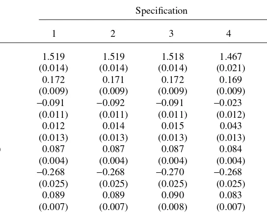
Covariate 1 2 3 4 5
Intercept 1.519 1.519 1.518 1.467 1.472
(0.014) (0.014) (0.014) (0.021) (0.021)
1 if male 0.172 0.171 0.172 0.169 0.169
(0.009) (0.009) (0.009) (0.009) (0.009)
1 if black −0.091 −0.092 −0.091 −0.023 −0.026
(0.011) (0.011) (0.011) (0.012) (0.012)
1 if Hispanic 0.012 0.014 0.015 0.043 0.040
(0.013) (0.013) (0.013) (0.013) (0.013) Cumulative years of work experience since age 20 (ACTX) 0.087 0.087 0.087 0.084 0.084
(0.004) (0.004) (0.004) (0.004) (0.004)
ACTX2/100 −0.268 −0.268 −0.270 −0.268 −0.267
(0.025) (0.025) (0.025) (0.025) (0.025) Cumulative years of work experience before age 20 0.089 0.089 0.090 0.083 0.083
(0.007) (0.007) (0.008) (0.007) (0.007)
No high school diploma, S≤8 −0.176 −0.176 −0.176 −0.111 −0.113
Light and Strayer
771
Master’s, doctorate or professional degree 0.047 0.046 0.050 0.019 0.036
(0.037) (0.038) (0.038) (0.037) (0.037)
Percentile score on AFQT/100 0.320 0.310
(0.025) (0.025)
Number of public, two-year colleges in state 0.001 0.001
per 100,000 residents age 18-26 (0.004) (0.004)
Number of public, four-year colleges in state −0.033 −0.032
per 100,000 residents age 18-26 (0.005) (0.005)
Cumulative duration of enrollment in two-year college (DUR2) 0.021
(0.010)
DUR22/100 −0.124
(0.087)
Cumulative duration of enrollment in four-year college (DUR4) 0.048
(0.014)
DUR42/100 −0.399
(0.133)
Root mean square error 0.538 0.537 0.537 0.533 0.533
R2 0.232 0.233 0.233 0.245 0.246
References
Altonji, Joseph G. 1993. “The Demand for and Return to Education When Education Out-comes Are Uncertain.” Journal of Labor Economics11(1, part1):48–83.
Brewer, Dominic J., Eric R. Eide, and Ronald G. Ehrenberg. 1999. “Does It Pay to Attend an Elite Private College? Cross-Cohort Evidence on the Effects of College Type on Earnings.”
Journal of Human Resources34(1):104–23.
Card, David. 1999. “The Causal Effect of Education on Earnings.” In Handbook of Labor Economics, Vol. 3A, eds. Orley Ashenfelter and David Card, 1801–63. Amsterdam: North-Holland.
Card, David, and Thomas Lemieux. 2001. “Can Falling Supply Explain the Rising Return to College for Younger Men? A Cohort-Based Analysis.” Quarterly Journal of Economics
116(2):705– 46.
Comay, Yochanan, Arie Melnik, and Moshe A. Pollatschek. 1973. “The Option Value of Edu-cation and the Optimal Path for Investment in Human Capital.” International Economic Review14(2):421–35.
Dale, Stacey Berg, and Alan B. Krueger. 1998. “Estimating the Payoff to Attending a More Selective College: An Application of Selection on Observables and Unobservables.” Quar-terly Journal of Economics117(4):1491–1528.
Grubb, W. Norton. 1993. “The Varied Economic Returns of Postsecondary Education: New Evidence from the Class of 1972.” Journal of Human Resources28(2):365–82.
Hilmer, Michael J. 1997. “Does Community College Attendance Provide a Strategic Path to a Higher Quality Education?” Economics of Education Review16(1):59–68.
———. 2000. “Does the Return to University Quality Differ for Transfer Students and Direct Attendees?” Economics of Education Review19(1):47–61.
Jaeger, David A., and Marianne E. Page. 1996. “Degrees Matter: New Evidence on Sheepskin Effects in the Returns to Education.” Review of Economics and Statistics78(4):733–40. Jones, Janis Cox, and Beth S. Lee. 1992. “Moving On: A Cooperative Study of Student
Trans-fer.” Research in Higher Education33(1):125–40.
Jovanovic, Boyan. 1979a. “Job Matching and the Theory of Turnover.” Journal of Political Economy87(5, part1):972– 90.
———. 1979b. “Firm-Specific Capital and Turnover.” Journal of Political Economy
87(6):1246–60.
Juhn, Chinhui, Kevin M. Murphy, and Brooks Pierce. 1993. “Wage Inequality and the Rise in Returns to Skill.” Journal of Political Economy101(3):410–42.
Kane, Thomas J., and Cecilia Elena Rouse. 1995. “Labor Market Returns to Two- and Four-Year College.” American Economic Review85(3):600–14.
———. 1999. “Community College: Educating Students at the Margin between School and Work.” Journal of Economic Perspectives13(1):63–84.
Katz, Lawrence F., and David H. Autor. 1999. “Changes in the Wage Structure and Earnings Inequality.” In Handbook of Labor Economics, Volume 3A, eds. Orley Ashenfelter and David Card, 1463–1555. Amsterdam: North-Holland.
Katz, Lawrence F., and Kevin M. Murphy. 1992. “Changes in Relative Wages, 1963–1987: Supply and Demand Factors.” Quarterly Journal of Economics107(1):35–78.
Kearney, Gretchen Warner, Barbara K. Townsend, and Terrence J. Kearney. 1995. “Multiple-Transfer Students in a Public Urban University: Background Characteristics and Interinsti-tutional Movements.” Research in Higher Education36(3):323–44.
Lee, Valerie E., and Kenneth A. Frank. 1990. “Students’ Characteristics that Facilitate the Transfer from Two-year to Four-year Colleges.” Sociology of Education63(3):178–93. Leigh, Duane E., and Andrew M. Gill. 1997. “Labor Market Returns to Community Colleges:
Evidence for Returning Adults.” Journal of Human Resources32(2):334–53.
The Journal of Human Resources
Light, Audrey. 1995. “The Effects of Interrupted Schooling on Wages.” Journal of Human Resources30(3):472–502.
———. 2001. “In-School Work Experience and the Returns to Schooling.” Journal of Labor Economics19(1):65 – 93.
Light, Audrey, and Wayne Strayer. 2000. “Determinants of College Completion: School Qual-ity or Student AbilQual-ity?” Journal of Human Resources35(3):299–332.
Loury, Linda Datcher, and David Garman. 1995. “College Selectivity and Earnings.” Journal of Labor Economics13(2):289–308.
Manski, Charles F. 1989. “Schooling as Experimentation: A Reappraisal of the Postsecondary Dropout Phenomenon.” Economics of Education Review8(4):305–12.
McCormick, Alexander C., and C. Dennis Carroll. 1997. “Transfer Behavior Among Begin-ning Postsecondary Students: 1989–94.” Statistical Analysis Report NCES97-266, National Center for Education Statistics. Washington, D.C.: U.S. Department of Education. Monk-Turner, Elizabeth. 1994. “Economic Returns to Community and Four-Year College
Education.” Journal of Socio-Economics23(4):441–47.
Rouse, Cecilia Elena. 1995. “Democratization or Diversion? The Effect of Community Col-leges on Education Attainment.” Journal of Business and Economic Statistics
13(2):217–24.
———. 1998. “Do Two-Year Colleges Increase Overall Educational Attainment? Evidence from the States.” Journal of Policy Analysis and Management17(4): 595–620.
Topel, Robert H., and Michael P. Ward. 1992. “Job Mobility and the Careers of Young Men.”
Quarterly Journal of Economics107(2):439–79.
Ureta, Manuelita, and Finis Welch. 1998. “Measuring Educational Attainment: the Old and the New Census and BLS Taxonomies.” Economics of Education Review17(1):15–30. Velez, W., and Rajshekhar G. Javalgi. 1987. “Two-year College to Four-year College: The