THE DEVELOPMENT OF
INDONESIAN VEHICLE OWNERSHIP MODEL
By
Leksmono Suryo Putranto1)
Abstract
As in any other developing country, in Indonesia there is an increasing degree of motorization. Transport policies such as high road investment expenditure, inadequate road user charging system and insufficient public transport services encourage the use of private vehicles. Vehicle ownership models are needed by the government for various purposes such as producing rough predictions of the demand on the highway network and consequent energy consumption, introducing appropriate transportation demand management, predicting income from car purchasing tax / car registration tax and the contribution of vehicle manufacturing industries to public wealth. Such models have been produced for several developing countries for decades but have not been comprehensively studied in Indonesia. The feature of the model proposed for Indonesia is motorcycle ownership as the intermediate vehicle ownership before owning a car. Aggregate models (municipality and regency based) will be developed using mostly secondary data obtained from the Indonesian Central Agency of Statistics (1991-2000) and other related government agencies. To provide basic knowledge of household vehicle purchase history, a limited retrospective multiple-cohort study based on a single cross-sectional survey will be conducted. Key Words : Vehicle Ownership, Indonesia, Aggregate Models, Cohort Study
1) Lecturer, Civil Engineering Department, University of Tarumanagara
I. INTRODUCTION
As in any other developing country, in Indonesia there is an increasing degree of motorization. High road investment expenditures, inadequate road user charges system and insufficient public transport services encourage the use of private vehicles.
Indonesia’s road sector consumes more than
7% of its GNP and more than 88% of passenger transport travels on the highway system, compared to only 5% on the railway system. Road expenditures have increased by five times between 1985-1991. Road expenditures have increased from 9% to 20%
of government’s overall budget These expenditures have not been compensated for by increases in road user charges. The user of road network is thus subsidized by the general taxpayer. A considerable percentage of subsidies is enjoyed by trucks, which account for more than 50% of the motorized vehicles on inter-urban roads and which
consume most of the heavily subsidized diesel fuel (World Bank, 1992 in Hook and Replogle, 1996).
Vehicle ownership models are needed by the government for various purposes such as producing rough prediction of the demand on the highway network and consequent energy consumption, introducing appropriate transportation demand management and predicting income obtained from car purchasing tax / car registration tax and contribution of vehicle manufacture industries to public wealth. Such models have been developed in many developing countries for decades but have not been comprehensively developed in Indonesia. A feature of the models required for Indonesia is motorcycle ownership as an intermediate stage of vehicle ownership before owning a car.
There are a lot of previous studies of vehicle ownership, concerning both modelling issues and the policy implications of the results of the model. Several factors were found to be affecting car ownership, as can be concluded from a study including 37 cities world-wide by Kenworthy and Laube (1999), a study including 26 countries world-wide by Dargay and Gately (1999), a study including USA and Netherland by Bhat and Pulugurta (1998), a study in Japan by Niiro (1987), several studies in the UK by Bates et al (1981), Hopkin (1981), Oldfield (1979) and Fowkes (1977), i.e.:
wealth (personal and regional) cost of vehicle ownership and use age structure of the population population density
public transport services
support to non-motorised transport road density
Factors affecting motorcycle ownership are similar with factors affecting car ownership, with several additional factors according to several studies in the UK by Broughton (1987), Hobbs et al (1986), and a study in the UK and the USA by Tanner (1977), i.e.:
weather topography
riding licence application procedure
Bhat and Pulugurta (1998) stated that car ownership modelling could be in the form of either aggregate or disaggregate models. In the aggregate model, car ownership is modelled at the aggregate level, e.g. zonal, regional or national level. In the disaggregate model, the household is used as the decision making unit and the forecasts at zonal, regional, or national level are obtained by aggregating over households. Oi and Shuldiner (1963) and Schor (1989) in Bhat and Pulugurta (1998) stated that the disaggregate models are structurally more behavioural compared to aggregate models and are better able to capture the causal
relationship between auto ownership
determinants and auto ownership levels.
III. STRUCTURE OF THE MODEL
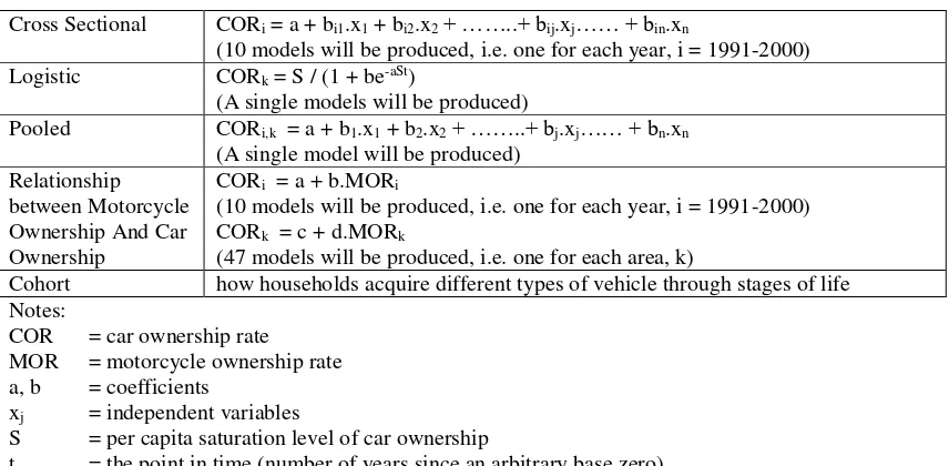
Only private car and motorcycle ownership will be considered in this model. There will be five broad categories of model. The purpose of equation description in each model is only to explain the included dependent and independent variables. The structure of the equations will not necessarily be adopted since the suitability of other equation forms will be statistically tested and boundary conditions such as the saturation level of vehicle ownership should be considered. Equation descriptions, which mention car ownership, only are applicable in the similar form in motorcycle ownership model as well. Those categories of models are listed in Table 1.
Regional characteristics that hypothetically have effects on vehicle ownership in Indonesia and the justification of their inclusion (besides data availability reason) are listed in Table 2. Three broad categories of independent variables will be considered, i.e. socio-economic, land use / transportation system availability and topography / climate. The last category will be used especially for motorcycle ownership modelling. Justifi-cation will be based either on previous research or logical reasoning.
IV. SAMPLING
done using lists of regencies and/or municipalities. Detail about the selection
process will be provided later.
Table 1. Type of Models
Cross Sectional CORi = a + bi1.x1 + bi2.x2 + ……..+ bij.xj…… + bin.xn
(10 models will be produced, i.e. one for each year, i = 1991-2000) Logistic CORk = S / (1 + be-aSt)
(A single models will be produced)
Pooled CORi,k = a + b1.x1 + b2.x2 + ……..+ bj.xj…… + bn.xn (A single model will be produced)
Relationship between Motorcycle Ownership And Car Ownership
CORi = a + b.MORi
(10 models will be produced, i.e. one for each year, i = 1991-2000) CORk = c + d.MORk
(47 models will be produced, i.e. one for each area, k)
Cohort how households acquire different types of vehicle through stages of life Notes:
COR = car ownership rate
MOR = motorcycle ownership rate
a, b = coefficients xj = independent variables
S = per capita saturation level of car ownership
t = the point in time (number of years since an arbitrary base zero)
Table 2. Independent Variables Included in the Model
Independent Variables Justification
Socio-Economic Variables:
Per Capita Income, i.e. Regional Income (RI) divided by mid year population of a region at the corresponding year. RI is the Net Regional Product (NRP) at market prices minus net indirect taxes (indirect taxes minus subsidies). NRP is the Gross Regional Product (GRP) subtracted by the total depreciation of fixed capital goods utilized in the production process. GRP is the sum of GRDP (Gross Regional Domestic Product) and the net factor income from abroad and from other regions. The net income from abroad and from other regions constitutes all income of production factors (labour and capital) owned by residents and accrued from abroad and from other regions, minus similar payments made to non-residents abroad and in other regions. (http://www.bps.go.id)
Per capita income is one of several wealth measures that can be used to express ability to purchase vehicle. Therefore, the higher the per capita income, the higher the vehicle ownership. However at certain level of per capita income the vehicle ownership may reach saturation and public transport service may theoretically satisfactory (due to the level of wealth reached). In that circumstance the growth of vehicle ownership may decline.
Consumer Price Index, i.e. an index that measures the average change in prices between times, of a package of goods and services consumed by the population/ households in a certain base period (http://www.bps.go.id)
Theoretically, the higher this index the lower the ability of individuals to purchase vehicle
Minimum Regional Wage This variable describe cohorts potentially own motorcycle
Percentage of population who has a job This variable is chosen to describe cohorts potentially own motorcycle or car
Independent Variables Justification
Percentage of population aged between 16 – 25 years This variable is chosen to describe cohorts potentially own motorcycle
Land-Use and Transportation System Availability Variables:
Population density per sq.km This variable express feasibility of providing comprehensive public transport system. The lower its value the higher the need to own private vehicle since mass public transport will not be feasible.
Road density, i.e. length of road (in km) divided either by land area or by population (Dargay and Gately, 1999)
Road density represents accessi-bility of private vehicle to travel using road network. The higher the road density the higher the accessibility. Higher accessibili-ty of private vehicle may encou-rage desire to own private vehicle.
Public transport service, i.e. in terms of static capacity of public transportation fleets per 1000 population
Theoretically, the better the public transport service the lower the private vehicle ownership.
Terrain and Climate Variables:
Average ground elevation above sea level High ground elevation of a region usually associated with hilly / mountainous terrain which theoretically associated with low motorcycle ownership if driving performance in terms of power to weight ratio is concerned. On the contrary, if vehicle manoeuvre flexibility in limited width of roads in hilly / mountainous terrain is concerned, then high motorcycle ownership may occur.
Average yearly rainfall (mm) Theoretically, the higher the yearly rainfall, the lower the motorcycle ownership.
V. THE DATA
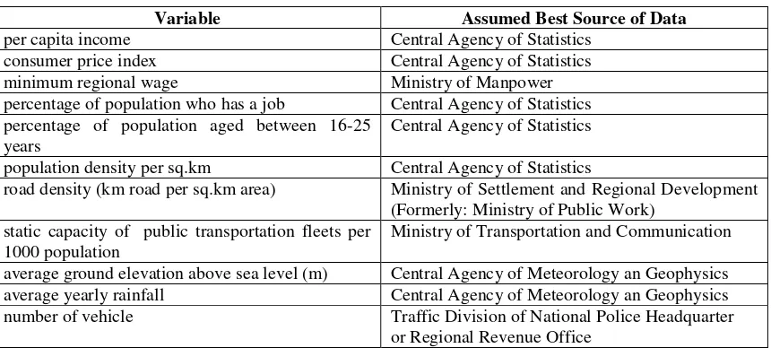
Main sources of data are official publication of Indonesian Central Agency of Statistics and Provincial Agency of Statistics. Most of the official publications are in the printed or books form, available in their libraries or bookshops. A limited amount of data can be
Table 3. Assumed Best Source of Data for Each Variable
Variable Assumed Best Source of Data
per capita income Central Agency of Statistics consumer price index Central Agency of Statistics minimum regional wage Ministry of Manpower percentage of population who has a job Central Agency of Statistics percentage of population aged between 16-25
years
Central Agency of Statistics population density per sq.km Central Agency of Statistics
road density (km road per sq.km area) Ministry of Settlement and Regional Development (Formerly: Ministry of Public Work)
static capacity of public transportation fleets per 1000 population
Ministry of Transportation and Communication average ground elevation above sea level (m) Central Agency of Meteorology an Geophysics average yearly rainfall Central Agency of Meteorology an Geophysics number of vehicle Traffic Division of National Police Headquarter
or Regional Revenue Office
Time period of data will be from 1991-2000 representing various socio-economic conditions of Indonesia, including period of economic crisis. However, critical selection of data should be made, since several yearly data are the result of applying certain growth factor on real census / survey data. The National Population Census is held every 10 year (e.g. in 1980, 1990, 2000), while in the middle of those ten years periods there are Intermediate National Population Surveys (e.g. in 1985, 1995). In the other years there are a lot of sector-based surveys (e.g. agricultural, industrial, trade and service, financial, price, etc) that are held regularly (in several sectors yearly) or incidentally.
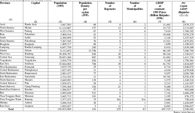
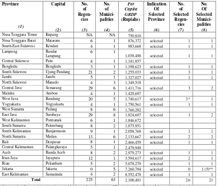
VI. DESCRIPTION OF STUDY AREA In order to understand the characteristics of the study area in general, Table 4. provides key information about 26 provinces in Indonesia. The former division of provinces is still used. The figure on column (8) will be used as one of selection criteria of the inclusion of a province in the research. Provinces having similar figure on column (8) will be represented by any province in the group in which the process of data collection will presumably be easier. Table 5. shows the application of criteria stated in section IV. and this section to determine selected province and number of regencies and number of municipalities that will be
included as sample from each of selected province. This table is sorted by per capita GRDP in ascending order. Selected province is indicated in column (6). In this case, provinces are grouped into classes of 100,000 wide per capita GRDP. Starting with Nusa Tenggara Timur in 700,000 – 799,999 class, following with Nusa Tenggara Barat in 800,000 – 899,999 class and so on. It should be noted that in 1,700,000 – 1,799,999 class, there are two provinces selected, i.e. West Java and Yogyakarta. It is difficult to choose one of them. West Java is very important province, since it has direct boundary to the capital of the state, Jakarta. Yogyakarta is important in this research, since it is well known as a bike or motorbike city. Although Nusa Tenggara Timur is the only member of 700,00 799,999 class, it is not selected, since it seems that the statistical office in this province will be difficult to be contacted.
Number of selected regencies is determined by using following criteria:
Number of
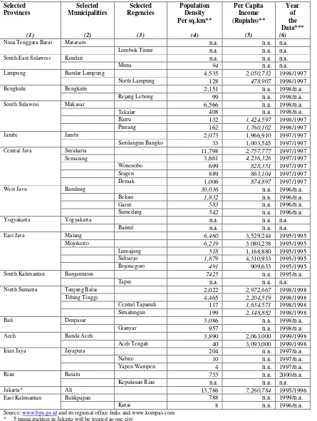
Number of regencies that will be included in the sample. The number of municipalities and regencies in selected provinces are based on Table 5. The selection was conducted using systematic sampling. Lists of municipalities and regencies obtained from www.bps.go.id, its link to regional statistical offices and Hill (1991) are assumed to be free from recurring patterns that required in systematic sampling (Fink (1995)). Population density and per capita income are used as municipalities and regencies characteristic indication. The
“n.a.” symbol does not necessarily mean no
data available at all. It indicates that recent data is not available. There will be a serious attempt to obtain such data during the data collection process.
VII. THE PLAN OF COHORT STUDY
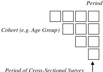
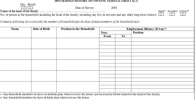
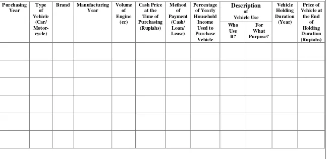
The purpose of a cohort study in this research is to develop an elementary model of behaviour of households on acquiring different types of vehicle through different stages of life. A Retrospective Multiple-Cohort Study Based on a Single Cross-Sectional Survey will be conducted. This type of cohort study is chosen since only single cross-section will be needed to obtain historical data of household vehicle purchasing behaviour (Mason and Fienberg, Ed., 1985). Therefore, both the practicability and the comprehensiveness of the study can be achieved. As can be seen in Figure 1, common age groups across cohorts can be linked by moving from the upper left to the lower right. The disadvantages of this design include memory decay in the respondents and as with other cross-sectional surveys we may simply be dealing with survivors. The preliminary design of questionnaire that will be used in the cohort survey is presented on Figure 2a and 2b.
Period
Cohort (e.g. Age Group)
Period of Cross-Sectional Survey
Figure 1. Retrospective Multiple-Cohort Study from Single Cross- availability of the contact person in the area. However, Table 7 shows that the selected areas have various characteristics of population density and per capita income.
The number of respondents in each regency and municipality will be 15, resulting in a total number of respondents of 90. Considering the limited number of samples, selected households should ideally have similar characteristics with average households in the related area in order to be representative.
Table 4. Description of Study Area
Province
(1)
Capital
(2)
Population (1995)
(3)
Population Density
per sq.km (1995)
(4)
Number of Regencies
(5)
Number of Municipalities
(6)
GRDP at constant 1993 Prices (Billion Ruipahs)
(1996) (7)
Per Capita GRDP (Rupiahs)
(7) / (3)
(8)
Aceh Banda Aceh 3,847,583 69 8 2 11,463 2,979,273
North Sumatra Medan 11,114,667 157 13 6 23,715 2,133,667
West Sumatra Padang 4,323,170 87 8 6 7,610 1,760,282
Riau Pekanbaru 3,900,534 41 5 2 19,808 5,078,279
Jambi Jambi 2,369,959 53 5 1 3,145 1,327,027
South Sumatra Palembang 7,207,545 70 8 2 13,521 1,875,951
Bengkulu Bengkulu 1,409,117 66 3 1 1,689 1,198,623
Lampung Bandar Lampung 6,657,759 200 6 1 6,914 1,038,488
Jakarta Jakarta 9,112,652 13,786 0 5 66,165 7,260,784
West Java Bandung 39,206,787 848 20 5 68,244 1,740,617
Central Java Semarang 29,653,266 867 29 6 41,862 1,411,716
Yogyakarta Yogyakarta 2,916,779 920 4 1 5,106 1,750,561
East Java Surabaya 33,844,002 706 29 8 61,752 1,824,607
West Kalimantan Pontianak 3,635,730 25 6 1 6,714 1,846,672
Central Kalimantan Palangkaraya 1,627,453 11 5 1 4,036 2,479,949
South Kalimantan Banjarmasin 2,893,477 77 9 1 5,957 2,058,769
East Kalimantan Samarinda 2,314,183 11 4 3 19,792 8,552,478
North Sulawesi Manado 2,649,093 139 4 3 3,575 1,349,518
Central Sulawesi Palu 1,938,071 28 4 1 2,213 1,141,857
South Sulawesi Ujung Pandang 7,558,368 104 21 2 9,486 1,255,033
South-East Sulawesi Kendari 1,586,917 57 4 1 1,561 983,668
Bali Denpasar 2,895,649 521 8 1 7,142 2,466,459
Nusa Tenggara Barat Mataram 3,645,713 181 6 1 3,195 876,372
Nusa Tenggara Timur Kupang 3,577,472 75 NA NA 2,686 750,810
Maluku Ambon 2,086,516 28 4 1 2,981 1,428,697
Irian Jaya Jayapura 1,942,627 5 12 1 6,983 3,594,617
Total 193,915,089 101 225 63 407,315 2,100,481
Table 5. Selected Provinces and Number of Regencies & Number of Municipalities Included in the Sample
Province
(1)
Capital
(2)
No. of Regen-
cies
(3)
No. of Munici-
palities
(4)
Per Capita GRDP (Rupiahs)
(5)
Indication Of Selected Province
(6)
No. of Selected
Regen- cies
(7)
No. Of Selected Munici- palities
(8)
Nusa Tenggara Timur Kupang NA NA 750,810
Nusa Tenggara Barat Mataram 6 1 876,372 selected 1 1
South-East Sulawesi Kendari 4 1 983,668 selected 1 1
Lampung Bandar
Lampung
6 1
1,038,488 selected 1 1
Central Sulawesi Palu 4 1 1,141,857
Bengkulu Bengkulu 3 1 1,198,623 selected 1 1
South Sulawesi Ujung Pandang 21 2 1,255,033 selected 3 1
Jambi Jambi 5 1 1,327,027 selected 1 1
North Sulawesi Manado 4 3 1,349,518
Central Java Semarang 29 6 1,411,716 selected 3 2
Maluku Ambon 4 1 1,428,697
West Java Bandung 20 5 1,740,617 selected 3* 1
Yogyakarta Yogyakarta 4 1 1,750,561 selected 1 1
West Sumatra Padang 8 6 1,760,282
East Java Surabaya 29 8 1,824,607 selected 3 2
West Kalimantan Pontianak 6 1 1,846,672
South Sumatra Palembang 8 2 1,875,951
South Kalimantan Banjarmasin 9 1 2,058,769 selected 1 1
North Sumatra Medan 13 6 2,133,667 selected 2 2
Bali Denpasar 8 1 2,466,459 selected 1 1
Central Kalimantan Palangkaraya 5 1 2,479,949
Aceh Banda Aceh 8 2 2,979,273 selected 1 1
Irian Jaya Jayapura 12 1 3,594,617 selected 2 1
Riau Pekanbaru 5 2 5,078,279 selected 1 1
Jakarta Jakarta 0 5 7,260,784 selected 0 1 (5)**
East Kalimantan Samarinda 4 2 8,552,478 selected 1 1
Total 225 63 2,100,481 26 21
Table 6. Municipalities and Regencies Included in the Sample
Selected Provinces
(1)
Selected Municipalities
(2)
Selected Regencies
(3)
Population Density Per sq.km**
(4)
Per Capita Income (Rupiahs)**
(5)
Year of the Data*** (6)
Nusa Tenggara Barat Mataram n.a. n.a. n.a.
Lombok Timur n.a. n.a. n.a.
South-East Sulawesi Kendari n.a. n.a. n.a.
Muna 94 n.a. n.a.
Lampung Bandar Lampung 4,535 2,050,732 1998/1997
North Lampung 128 478,907 1998/1997
Bengkulu Bengkulu 2,151 n.a. 1998/n.a.
Rejang Lebong 99 n.a. 1998/n.a.
South Sulawesi Makasar 6,566 n.a. 1998/n.a.
Takalar 408 n.a. 1998/n.a.
Barru 132 1,424,597 1998/1997
Pinrang 162 1,760,102 1998/1997
Jambi Jambi 2,073 1,966,910 1997/1997
Sarolangun Bangko 33 1,003,545 1997/1997
Central Java Surakarta 11,798 2,757,777 1997/1997
Semarang 3,661 4,236,326 1997/1997
Wonosobo 699 828,351 1997/1997
Sragen 889 863,104 1997/1997
Demak 1,006 874,897 1997/1997
West Java Bandung 30,036 n.a. 1996/n.a.
Bekasi 1,832 n.a. 1996/n.a.
Garut 583 n.a. 1996/n.a.
Sumedang 542 n.a. 1996/n.a.
Yogyakarta Yogyakarta n.a. n.a. n.a.
Bantul n.a. n.a. n.a.
East Java Malang 6,460 3,529,244 1995/1995
Mojokerto 6,219 3.080,238 1995/1995
Lumajang 518 1,168,880 1995/1995
Sidoarjo 1,879 4,310,933 1995/1995
Bojonegoro 491 909,633 1995/1995
South Kalimantan Banjarmasin 7425 n.a. 1995/n.a.
Tapin n.a. n.a. n.a.
North Sumatra Tanjung Balai 2,022 2,972,667 1998/1998
Tebing Tinggi 4,465 2,204,519 1998/1998
Central Tapanuli 117 1,634,571 1998/1998
Simalungun 199 2,148,882 1998/1998
Bali Denpasar 3,086 n.a. 1998/n.a.
Gianyar 957 n.a. 1998/n.a.
Aceh Banda Aceh 3,890 2,063,000 1999/1998
Aceh Tengah 40 3,093,000 1999/1998
Irian Jaya Jayapura 204 n.a. 1997/n.a.
Nabire 10 n.a. 1997/n.a.
Yapen Waropen 4 n.a. 1997/n.a.
Riau Batam 755 n.a. 2000/n.a.
Kepulauan Riau n.a. n.a. n.a.
Jakarta* All 13,786 7,260,784 1995/1996
East Kalimantan Balikpapan 788 n.a. 1999/n.a.
Kutai 8 n.a. 1996/n.a.
Source: www.bps.go.id and its regional office links and www.kompas.com * 5 municipalities in Jakarta will be treated as one city
** Estimated data are printed in italic
Table 7. Municipalities and Regencies Included in the Sample
Lampung Bandar Lampung 4,535 2,050,732 1998/1997 Central Java Semarang 3,661 4,236,326 1997/1997
West Java Bekasi 1,832 n.a.* 1996/n.a.
Garut 583 n.a.* 1996/n.a.
Yogyakarta Bantul n.a. n.a. n.a.
Jakarta All 13,786 7,260,784 1995/1996
Source: www.bps.go.id and its regional office links
5 municipalities in Jakarta will be treated as one city + Estimated data are printed in italic
* Estimated per capita GRDP in West Java was 1,740,617 in 1996
Estimated per capita GRDP in Yogyakarta was 1,750,561 in 1996
# First figure for population density year, second figure for per capita income year
Descriptive statistics will be produced to provide a general description of the characteristics of household, vehicle ownership and vehicle use in each selected regency and municipality. These will include the mean, standard deviation, median and mode of the following current attributes:
Number and age of household
Number of servants in the household Number, age, and engine size of cars
owned
Number, age and engine size of motorcycles owned
The other descriptive statistics that will be produced are the mean, standard deviation, median and mode of the following historical attributes:
Holding durations of any cars owned during the life of the household Holding durations of any motorcycles
owned during the life of the household
The models will mainly describe
relationships between following pairs of attributes: of motorcycles owned/number of household members
Several cross tabulations showing percentage distribution of certain pairs of vehicle ownership characteristics will also be produced, e.g. between:
Brand, engine size and vehicle use Brand, engine size, manufacturing
year, cash price at the time of purchasing, method of payment and percentage of yearly household income used to purchase vehicle Brand, engine size, manufacturing
year, vehicle holding duration and price of vehicle at the end of holding duration
Figure 2a. Preliminary Design of Cohort Survey Questionnaire (Sheet 1)
HOUSEHOLD HISTORY ON OWNING VEHICLE (Sheet 1 of 2) Day Month
Date of Survey: 2001
Name of the head of the family: ……….. main+ servants visitors#
No. of person in the household (including the head of the family; including any live-in servants and any other long term visitors):
Complete following list to describe the member of household (put the data of main members of the household only)
Name Date of Birth Position in the Household Employment History (If Any)*
Year Position
From To
+ Any household members ho have no definite plan when to leave the house, not necessarily blood related to the head of the family x Any household members ho have definite plan when to leave the house
* Start from the latest and include all money earning activities (running own business, self employed profession, etc.)
Figure 2b. Preliminary Design of Cohort Survey Questionnaire (Sheet 2)
HOUSEHOLD HISTORY ON OWNING VEHICLE (Sheet 2 of 2)
Complete following list to describe the household history of purchasing vehicles .Please start from the vehicle purchased earliest.
Purchasing Year
Type of Vehicle
(Car/ Motor-
cycle)
Brand Manufacturing Year
Volume of Engine
(cc)
Cash Price at the Time of Purchasing
(Rupiahs)
Method of Payment
(Cash/ Loan/ Lease)
Percentage of Yearly Household Income Used to Purchase
Vehicle
Description of Vehicle Use
Vehicle Holding Duration
(Year)
Price of Vehicle at
the End of Holding Duration (Rupiahs) Who
Use It?
VIII. CONCLUDING REMARKS analysis of missing values, especially when general model is going to be built. Developing more specific models based on certain characteristics might be useful to minimize the impact of missing values. It will also be possible to replace the selected municipalities or regencies in which incomplete data sets mostly found.
The reliability of the secondary data can also be serious problem. For the same type of data, different institution may provide different value of data. Therefore past experience of recognized researchers in this field in Indonesia about the best source of each type of data should be considered. An attempt to check the reliability of certain data type by comparing these data with the reliable data from other type can also be done. For example, if it is believed that GNP per capita data is reliable, it can be used as a logical comparison to the car ownership data sets. In this case we should doubt the reliability of the data if in a very low GNP per capita area, there is a very high car ownership rate.
Another type of problem may occur during cohort survey. Some respondents may feel reluctant to answer several sensitive questions such as income and vehicle use. The interviewer should be well trained to avoid complete refusal. He or she should be able to persuade the respondent to provide at least essential information, although detail information may not be obtained.
REFERENCES
Bates J., et al (1981). The Factors
Affecting Household Car
Ownership. Gower Publishing Limited, Westmead.
Bhat, C. R., Pulugurta, V. (1998). A Comparison of Two Alternative Behavioral Choice Mechanism for
Household Auto Ownership
Decisions. Transportation
Research Part B Vol. 32 No.1, 61-75.
Broughton, J. (1987). The Effect on Motorcycling of the 1981 Transport Act. Research Report 106, Transport and Road Research Laboratory, Crowthorne.
Button, et al (1982). Car Ownership Modelling and Forecasting. Gower
Publishing Company Ltd.,
Alderrshot.
Dargay, J., Gately, D. (1999). Income’s Effect on Car and Vehicle Ownership, Worldwide: 1960-2015. Transportation Research Part A 33, 101-138.
Fink, A. (1995). How to Sample in Survey. Sage Publication, Inc. London
Fowkes, A. S. (1977). Initial Investigation of the Wytconsult Household Survey Data for Illustrating
Methods of Car Ownership
Forecasting. Working Paper 96, Institute for Transport Studies, University of Leeds.
Hook, W., Replogle, M. (1996). Motorization and Non-Motorized Transport in Asia: Transport System Evolution in China, Japan and Indonesia. Land Use Policy Vol. 13, No.1, 69-84.
Hopkin, J. M. (1981). The Ownership and Use of Cars by Elderly People. . TRRL Laboratory Report 969. Transport and Road Research Laboratory, Crowthorne.
Kenworthy, J. R., Laube, F. B. (1999).
Patterns of Automobile
Dependence in Cities: An
International Overview of Key
Physical and Economic
Dimensions with Some
Implications for Urban Policy. Transportation Research Part A 33 (1999), 691-723.
Mason, W. M., Fienberg, S. E. (Ed.) (1985). Cohort Analysis in Social Research. Springer-Verlag New York Inc. New York.
Niiro, K. (1987). The Impact of Public Transport Service on Regional Car Ownership and Passenger Demand. Thesis (M.Phil.) Department of Economic Studies, University of Leeds.
Oldfield, R. H. (1979). Effect of Car Ownership on Bus Patronage. Laboratory Report 872, Transport and Road Research Laboratory, Crowthorne.
Tanner, J. C. (1977). Trends in Motorcycle
Ownership and Use. TRRL
Supplementary Report 361.
Transport and Road Research Laboratory, Crowthorne.