didiks IJABER Vol.15 N0.3 2017 pp.17 42 Publikasi Profesi Unsri (1) (1)

(1)

Expenditure Analysis of Local Government and Regional Economic Development District/City of Ten Province in...

Expenditure Analysis of Local Government and Regional Economic

Development District/City of Ten Province in Sumatra Island

Indonesia

Didik Susetyo

1

_{, Zunaidah}

2

_{, Siti Rohima}

3

_{, Anna Yulianita}

4

_{, Mohamad Adam}

5*

_and

Devi Valeriani

6

1-5_{Lectures of Economic Faculty of Sriwijaya University} 6_{Lecture of Economic Faculty of Bangka Belitung university} * Coressponding Author: mr_adam2406@yahoo.com

Abstract: The research problem is how to influence the local government spending, the number of local civil servants (PNSD), and the number of regional infrastructure to the local economic development districts/ cities in Sumatra island of Indonesia. While the purpose of the study is to estimate the model and analyze the influence of local government spending, the number of the civil servants, and the amount of infrastructure to the local economic development districts/cities in Sumatra island of Indonesia.Regional economic theory used is Keynesian model: Y = C + I + G + (X – M); A concept of Local Government Expenditure (local government spending) according to Wagner’s Law, Theory Peacock and Wiseman, Wagner, and Solow. While previous empirical research, among others is: (a) Susetyo (2003) and (b) Yanizar (2012).

Research methods include: (a) the scope of the studies in this research is local government spending, the number of local officials (PNSD), local infrastructure (road length), and the regional gross domestic product (local economic). The location of observation as the unit of analysis is the district/city as much as 155 (comprising 121 districts and 34 cities) on the island of Sumatra, Indonesia; (b) The data type and data source, that the type of data used are secondary data and are equipped with primary data analysis uni; (c) The method of analysis in this research is quantitative descriptive and equipped with qualitative descriptive.

(2)

Didik Susetyo, Zunaidah, Siti Rohima, Anna Yulianita, Mohamad Adam and Devi Valeriani

Simultaneously (F-test) showed that the results obtained are the three variables observed were local spending, the number of civil servants districts/cities, length of roads in the district/city catastrophically affect positively and significantly. This value amounted to 317.2543 F-statistic is greater than F-table so the independent variable positive and significant effect to dependent variable, with the result of random effect model estimation. Partially (t-test), indicating that the effect of local spending to the regional gross domestic product is positive and significant. The value t-statistic of the local spending, the number of civil servants, the length of the local road each 17.85835; 12.79292; –2.482922 are greater than t-table so that a positive and significant influence.Coefficient of determination (R2_{) is 0.506860, or 50.68 percent and Adjusted R}2_{= 50.52 percent,} means that the results can be explain by the model estimates a third variable and significant amounted percent, while the rest, or by 49, 32 percent is explained by factors outside the model. The best model after the Chow and Hausman test as well as the number of time series is less than the number of districts/cities, the best estimation models are models of random effect.

Keywords: local economic development (GRDP), the local spending, the number of local civil servant, long road, district/city.

I. INTRODUCTION

1.1. Background

The phenomenon that emerged on local government spending today in Indonesia still seem not optimal characterized by unfulfilled principles of efficiency, effectiveness, transparency, and accountability in the local fiscal. It seems that the application of the principles of management of local government spending is difficult to categorize good, let alone excellent. It is certainly no processes that lead to optimal management of local spending not yet reached the optimal category in terms of efficiency and effectiveness. “The overlap between levels of local government spending on discretionary possible development planning at local government level is less effective in its implementation” (Ministry of Finance, 2008).

Some aspects were identified affect the optimal management of local spending include the limited capability of the officers (civil servant), committed leadership in managing the local spending, and the condition of local infrastructure is inadequate. Empirical conditions shows that the management of local spending still preferred to drive local economic growth, but still meet the operational needs of the apparatus, especially the new autonomous regions (autonomous regions). One of the principleof the allocation of local spending to encourage economic growth in the region, in addition to increasing employment opportunities and poverty alleviation (Mardiasmo, 2002; Susetyo, 2003).

In connection with the phenomenon that local government spending has not fully improve the regional economic development is the focus of study in this research. On the one hand, there is a causal relationship between the local spending with the regional economic development. Likewise, that the study was expanded to model the effect of local spending, the number and capability of the officers, and the condition of local infrastructure to regional economic development.

1.2. Roadmap Research

(3)

regional economic growth. It means the relevance between university research plan with regional economic development into one of the research studies that have implications for the progress and welfare of the community.

This research activity is a continuation of previous stages of research that focuses on aspects of the revenue and local spending to encourage economic growth in the region. The research to be conducted is to analyze aspects of the local spending, the capabilities and the number of personnel, and the condition of the infrastructure to regional economic progress in an estimation model. This research activity is based on the current actual phenomena that some locals do spending without taking into account the impact of the principles of budget management more efficient and effective.

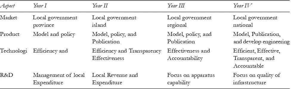
Related to the above, this research activity has a close connection between the four fundamental aspects of the roadmap of university research (RIP UNSRI, 2012) which markets, products, technology, and research and development (R&D) in this research activity can be showedto the roadmap of research in Table 1.

Table 1

Fiscal Management Research Roadmap Regional and Economicdevelopment District/City in Indonesia

Aspect Year I Year II Year III Year IV

Market Local government Local government Local government Local government

province island regional national

Product Model and policy Model, policy, and Model, policy, and Model, Publication, Publication Publication and develop engineering Technologi Efficiency and Efficiency and Transparency Effectiveness and Efficient, Effective,

Effectiveness Accountability Transparent, and Accountable R&D Management of local Local Revenue and Focus on apparatus Focus on quality of

Expenditure Expenditure capability infrastructure

1.3. Problems and Objectives

The research problem is how does local government spending, the number of local officials (PNSD), and the amount of local infrastructure (road length) to the development of the regional economy (GRDP) districts/cities in Sumatra island of Indonesia. In line with the research problem, the research objective is to analyze the effects of local government spending, the number of local officials (PNSD), and the amount of infrastructure (road length) on the development of the regional economy (GDP) districts/cities ten provinces in Sumatra Island of Indonesia.

1.4. Implementation Results Activity

Application of the results of these activities can be either conceptual references (modeling) and to do community service activities, especially the workshop, FGD, and Training on the importance of managing local government spending is efficient and effective. Means the application of the results of these activities can be performed:

(4)

Didik Susetyo,Zunaidah, Siti Rohima Anna Yulianita,Mohamad Adam and Dev i Valeriani

(b) Practically; form of training personnel/local human resource, improving the quality of infrastructure and policies for the management of local government revenue and expenditure in an efficient, effective, transparent, and accountable.

1.5. Outcomes and Contributions

Outcomes and contribute to the development of science and technology of the research activity include: (a) Document the results in the form of the model estimates, publications and scientific journals for

publication, both journals of international and national journals;

(b) Document the results of this study can be used as a reference or a reference in the formulation of policies and develop concepts in a model related to the management of local government revenue and expenditure.

II. STUDY REFERENCES 2.1. The Concept of Regional Economic

In macro regional economic activity may be indicated by the behavior of the economy in a market economy, the government, households, and businesses. All three of these principals perform economic activities with the objective of each specific and cumulatively can see their performance. By examining the activity of economic agents in the market can be obtained by several indicators, such as economic growth, inflation, labor market conditions, and the balance of trade in the economy. As such, regional economic activity can be seen from the development of the Gross Regional Domestic Product (GRDP) of each region as a whole.

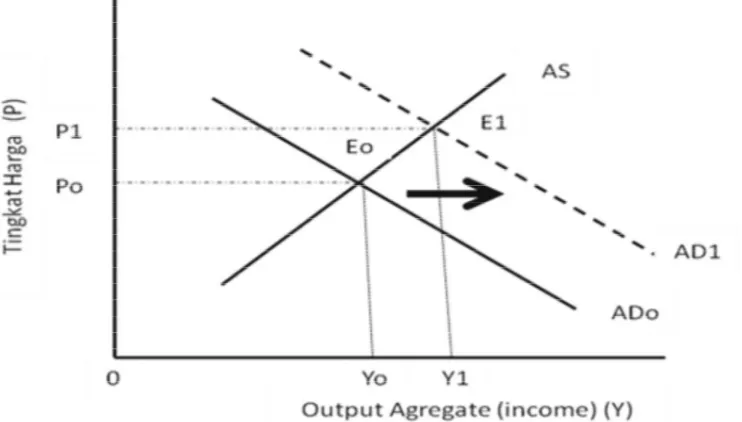
Macroeconomic policies according to Branson and Litvack (1981) is an instrument that is often used in developing policies that will affect the macro economy can be grouped into three, namely the implementation of fiscal policy by increasing government spending, the implementation of fiscal policy by cutting taxes, and monetary policy by increasing the money supply. Changes in the economy can be approximated by the instrument balance aggregate supply (AS) and aggregate demand, AD). The instrument can explain the condition of an economy that describes fluctuations in output, the price level, income level, and inflation. Figure 2.1 illustrates the interaction between aggregate demand and aggregate supply in the market (Dornbusch et. al., 2004, and Case and Fair, 1999).

Illustration Figure 2.1 shows that the point E₀ is the point of balance between the level of output and the price level. Shifting one curve for any reason will change the price level and output level. Aggregate demand curve shifts to the right can be caused by two things:

1. an increase in government spending, and 2. a decrease in taxes.

(5)

Aggregate Supply curve in concept is the curve that connects between the amount of goods and services offered by the company at a certain price. This curve slope is positive because the company always strives to offer the goods produced at a higher price. While the aggregate demand curve negative slope because higher prices would reduce the value of money supply which in turn will reduce the demand for the output. Aggregate demand curve is a curve that connects a combination of price levels and the level of output at an output markets and money markets simultaneously and the state of the market is in a state of balance (Mankiw, 2003).

In the modern economy, the components of aggregate demand consist of four indicators, namely: 1. household consumption expenditure,

2. the company’s investment expenditure, 3. the government spending, and

4. net exports (Krugman and Obstfeld, 2003).

This means that functionally, the government can develop policies that can affect the aggregate demand curve shifts. Components of aggregate demand should be managed optimally for a balance quality market. Thus, the area of macro-economic analysis needs to pay attention to such components. According to Krugman and Obstfeld (2003) that the aggregate demand mathematically formulated as follows.

– +++, – ...(1)

Where,

C (Y – T) = Consumption as a function of disposable income I + G = Investment and government spending (exogenous)

CA(EP */P, Y – T) = Current account that is a function of the real exchange rate anddisposable income Figure 2.1: Relations Price Level, Output, Aggregate Demand and Aggregate Supply

(6)

Didik Susetyo,Zunaidah, Siti Rohima Anna Yulianita,Mohamad Adam and Dev i Valeriani

The formula means that aggregate demand will be greatly affected by the amount of consumption that is a function of disposable income, tax, investment, government spending, and the exchange rate. Thus, investment and government spending is an exogenous factor that is important in moving the economy. In the regional economy, a more comprehensive analysis can be done by combining the IS-LM curve analysis with analysis of AD-AS. In the context of increasing investment and government spending analysis tools above can be used. Policy of increasing investment and government spending with the other held constant it will result in market balance shifted. The increase in investment resulted in a change similar to the change in government spending if the assumption is the LM curve remains, and there are no exports and imports in an economy. With the economy only consists of three sectors, namely the government, companies and households, the increase in government spending or increased investment will provide the same changes, namely the movement of IS to the right (Branson and Litvack, 1981).

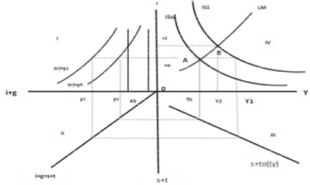
Illustration in Figure 2.2 that the increase of governments spending shift into g₁ from g₀. Under these conditions the output at every interest rate becomes higher. On the curve g₁ if the interest rate r₀, then the output achieved in conditions of balance is Y₁. So increased government spending affect the IS curve shifts to the right, ie from IS₀ to IS₁ curve. This means that the output becomes greater. Large output level will increase economic activity. Furthermore, these conditions will promote employment, will further reduce unemployment.

The illustration in Figure 2.2 above explains that r is the interest rate, y is the output, s is the savings, t is the tax, i is an investment, and g is government spending. In the same context, if the interest rate is lower than before, the investment will increase. By the same mechanism, the lower interest rates will also

(7)

increase output. Thus, the amount of investment and government spending has the same effect on the economy, namely the addition of output. This means that investment and government spending becomes strategic to improve the performance of the regional economy.

Economic performance is generally measured an area of economic growth is the increase in the value of goods and services produced by the region in a given time period. Economic growth is usually measured by the change in Gross Regional Domestic Product (GRDP) in percent real. The GDP is usually calculated with three approaches that conception would yield the same value the production approach, expenditure approach, and income approach. Mathematically, where, Yi is a sector GDPi, in year t as follows:

= 1, = 1, 2, 3, ..., ...(2)

Furthermore, to GDP (national) and the GRDP (local) by expenditure are all components of final demand, namely private household consumption and government consumption, investment and net exports, as identity can be seen as follows:

Y = C + I + G + (X – M). ...(3)

The above equation shows that the Y is GDP, C is private consumption and private, I was spending private investment, G is government spending and investment, X is exports and M is imports.

For GDP by income is the amount of compensations to production factors which participate in the production process in the form of wages and salaries, rent for land, capital interest, and profit before income tax and other direct taxes. In this definition, GDP includes depreciation and net indirect taxes (indirect taxes less subsidies).

The competent institution calculates the GDP and the GDP is the Central Statistics Board (BPS) on a regular basis every year. GDP data source production comes from departments or agencies that collect data on production, producer prices, the cost to produce, and expenses. In the context of smaller regions, namely provincial and district/city, economic growth is calculated using Gross Regional Domestic Product (GRDP), which reflects the region’s ability to manage its resources.

2.2. The concept of Local Government Spending

Local government spending is often called regional spending is a function of the reception area. The more increasing of local government is on revenue, the greater will the level of expenditure. This means that, the greater the revenue or acceptance, then the policy development of regional spending should plan spending appropriately and according to the needs of society in order to benefit from the budget can be more efficient and effective.

In the concept of regional spending is issued and the amount of funds used to finance all regional needs either requirement included in direct expenditure and included in indirect expenditures. Government spending (government expenditure) in practice is all purchases of goods and services performed by central and local governments. Government spending variables included in the group in which the magnitude of change exogenous value depends on the strategy adopted by local governments in implementing fiscal policy.

(8)

1. The development model of the development of government spending; 2. The Wagner Law concerning the development of the government’s activities;

3. Theory of Peacock and Wiseman. Explanation of the theory can be described as follows:

(a) Model of Government Spending

The development model of government spending is developed by Rostow and Musgrave. This model connects the development of government spending with economic development stages, ie the initial stage, intermediate stage and advanced stage. Stage in regional development is closely connected with the stage of economic development. Each stages of economic development has different focus of government spending but still have to pay attention to sustainability.

This is in line with the views expressed by Rostow and Musgrave in Mangkoesoebroto (2001) stated that in the early stages of economic development in government spending should provide infrastructure, such as education, health, infrastructure of transportation, and so forth. Therefore, in this stage the percentage of government investments made very large. At the intermediate stage of economic development is characterized by government spending focused on increasing economic growth in order to take off. Thus the government investment is still required in order to support in order to increase economic growth. At this stage is already greater private investment so that the role and contribution of the private sector in development is relatively larger than the first phase.

At the next level of government activity switch from the provision of infrastructure to expenditures for social activities such as programs for the elderly, programs for health services. This opinion gives an understanding that construction spending should be a concern primarily by the government itself in order allocated budget could be targeted in accordance with the plan that has been set so that the target can be realized. In the end the people’s welfare can be achieved as expected. However, based on research results Ramsey (2011) there was no government spending has a multiplier effect that follows a direct effect itself.

(b) Wagner law

Wagner’s Law is a law linking government spending to gross domestic product growth. Wagner law formulated government activity in development (Peters, 2012). Then, Atkinson and Stiglitz (1980) in Henrekson (1993) says that Wagner’s Law, known as “The Law of Expanding State Expenditure” in principle says that in the long term there is a tendency of the public sector will grow relative to national income. In other words, the development of greater government spending is as a percentage of Gross National Product (GNP).

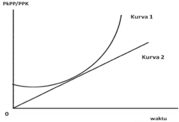
In this case Mangkoesoebroto (2001) says that in an economy where per capita income increased in relative terms, the government spending will also increase. Wagner’s Law is formulated as follows:

11 < 22 < ... < ...(4)

Where,

PkPP = government spending per capita PPK = Income per capita

(9)

The illustration in Figure 2.3 explains that the increase in government spending has the shape is not linear but exponential shape. The exponential form of the curve is shown by the curve 1 and not the curve 2. In economic growth increasingly large and complex, hence the greater industrial relations, relations between industry and the public is also more complicated and complex. Thus the role of government becomes even greater because the government must regulate relations arising in society, law, education, culture, health and so on. This could take place if the government considers as free individuals acting apart from the other members (Mangkoesoebroto, 2001).

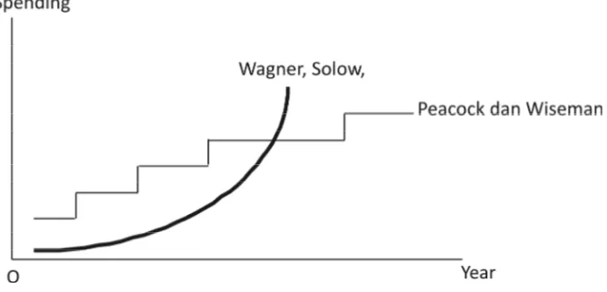
(c) Theory of Peacock and Wiseman

Peacock and Wiseman (1961) suggested that the development of government spending based on the view that the government is constantly trying to increase spending, while people do not like paying taxes to finance growing government spending them. Peacock and Wiseman stated that people have a tolerance level of the tax or the level of people’s willingness to pay taxes. The tolerance level of this tax is an obstacle for the government to raise the tax levy arbitrarily.

In more detail the theory of Peacock and Wiseman (Mangkoesoebroto, 2001) stated that economic development causes increasing tax collection though tax rates have not changed; and increased tax revenues caused government spending also increased. Therefore, under normal circumstances, the increase in GNP led to greater government revenues, as well as government spending becomes.

If the normal state is interrupted, for example because of the war, the government must increase spending to finance the war. Because of the government’s revenue from taxes also increased where an increase is obtained by increasing the tax rates that private fund for investment and consumption to be reduced. This condition is called diversion effect (displacement effect), namely the existence of a disorder that causes private activity shifted to government activity. This theory is illustrated in Figure 2.4.

(10)

In normal conditions, aside from increased taxes, the government also had to borrow from other countries with the consequences should return the loan principal and interest. Once the abnormal condition is over, there is a state called the effect of inspection. Effects inspection activities is the new government looks after the situation returned to normal. In addition, the social disorder will also cause some of the activities previously carried out by the private sector to the government concentrated (concentration effect). The third effect of the above lead to increased activity of the government after the situation returned to normal (war is over), so that the tax rate does not fall back as the level before the war.

In contrast to Wagner’s view, that the development of government spending versions of Peacock and Wiseman did not form a line, but shaped like a staircase as seen in Figure 2.5.

In relation to the local or regional financial, the full local potential and revenue called fiscal capacity. While total expenditure is called fiscal needs. The difference between the local fiscal capacity and the need for fiscal shows the magnitude of the local fiscal gap. The greater negative value of the fiscal gap shows more the regional fiscal disparities gap.

Figure 2.5: Development Curve of Government Spending Source: Mangkoesoebroto, 2013

(11)

Regional government spending cannot be separated from the local revenues, because theoretically the expenditure is a function of the local revenues. The higher the local revenuesaffect the higher level of local spending. For that area seeks to increase local revenues by trying to increase the source revenue and equalization funds. This has encouraged the local government tried to increase revenue potential through increased its revenue to be used for local spending within the framework of regional development.

In the process of government spending is the policy of the government to finance the construction of this area is included in the cost of the regional administration. In other words, local government spending is spending that is used to finance development in various fields, including in this case is the social, economic, governance, culture, order, tranquility, and so that is the task of government in general. In the area of financial management, governance of the administration often experience very significant changes in each period. It is adapted to the changing environment and system of government. Local spending held by the guidelines fo the Minister of the Home Affair No. 13/2006 (Regulation No.13 / 2006).

In Grand Design of Fiscal Decentralization (Ministry of Finance, 2008) stated that mission associated with local spending, namely:

1. Develop flexibility local spending responsible for achieving minimum service standards, 2. harmonization of centers expenditure and local spending to provide public services optimally. In detecting optimizing management of local spending can be seen how the influence of the presence and capabilities of human resources of the local apparatus (officials) and local infrastructure conditions. Potential regional civil servant as a proxy for labor which provides public services to the society, while the availability of local infrastructure as a proxy for direct investment requirement for the infrastructure to encourage the development of regional economy. This is certainly related to the road map research covering the stages of activities to be undertaken in a few years (multiyear research).

In line with the road map, the activity of this research is a series of research activities in the area of fiscal management that is efficient, effective, transparent and accountable. Activities that have been studied previously, among others, fiscal capacity and fiscal needs of the local area, then analyze the activities to be carried out on the management of local government expenditures and their implications for regional economic growth. The road map will be continuous research along with the development and progress of the region in managing local finance ever-increasing numbers, such as Wagner law (Soeparmoko, 2003).

In this study some novelty activities are expected to be revealed and proved from the study include: 1. local government spending patterns still dominant to finance operational expenditures (indirect

expenditure);

2. a shift in spending patterns will occur when the local government financial management has reached ten years;

3. a comparison between districts/cities reflect the diversity of the management of local government spending patterns;

(12)

2.3. Previous Research

Several previous studies that are relevant include: Susetyo (2003) examines the Analysis of Fiscal capacity and needs of Districts/Cities in Indonesia found the formulation of a model of regional spending as follows:

TPD/PDRB_it= –0.011003 + 0.000764 LogPDDK_it + 0.000449 LogPdat_it (–6.657039)**(3.122829)** (3.703719)** + 0.018945TKEM_it + 0.121645TPD/PDDK_it + 0.975354TPD/PDRB_i,t-1 ...(5)

(10.18361)** (35.1513)** (159.6705)**

Adj R-Sqr = 0.909632; SE of Reg = 0.017318; D-W stat = 1.778474; (t-value) where:

Pddk = total population, Pdat = density, Tkem = poverty, TPD/Pddk = ratio of local spending per capita, TPD/PSRBt–1 = ratio local spending the previous year, and TPD/GRDP = ratio of fiscal local

spending per GRDP,

Further research by Yanizar (2012), which is examined the impact of spending policy regional development funds and private investment to the GRDP and poverty in the Province of Jambi. Research is done by building a system of simultaneous equations econometric model using time series data from 1985 to 2010 year. The results of the research concluded that the cooperation between local governments and the private sector is essential for the economic development of the Province of Jambi due to limited fiscal capacity. This conclusion is based on findings which increase local government spending followed an increase in private investment in productive sectors will spur economic growth which in turn will reduce the level of poverty. Moreover, the consequences of the implementation of fiscal decentralization policy that allows the local governments to raise local revenue mainly from local taxes should be best utilized to develop the potential of receiving and allocating funds to the productive sectors and in the regions in an efficient and effective way to spur economic growth will increase revenue and decrease the number of poor people.

Based on the reference theory and previous research, the research framework can explain the relationships between concepts or variables that are formulated in a model. The model will be built in research activities can be seen in Chart 1.

Chart 1: Conceptual Framework Research

(13)

III. RESEARCH METHODS

3.1. Scope

The scope of the study in this research is local government spending, personnel capabilities (civil servants), local infrastructure (length of road) and local economic growth (GRDP). The location of observation as the unit of analysis is the districts/cities in Sumatra Island of Indonesia. The observation period is about 2010-2015.

3.2. Types and Sources of Data

The data used is secondary data and are equipped with primary data analysis unit. Secondary data sources are from the official publication of Directorate General Budget-Minister of Finance (DJA-Kemenkeu), the Central Board of Statistic (BPS), Local Planning Board (Bappedakabupaten/kota) and related Satuan Kerja Perangkat Daerah (SKPD).

3.3. Methods of Analysis

The method of analysis in this research is quantitative descriptive and equipped with qualitative descriptive. Parameter estimation method is used a multiple regression analysis (Multiple Ordinary Least Square).

Formulation of a mathematical model to be estimated is:

Y = f (X₁, X₂, X₃) ...(6)

Furthermore, an econometric model to estimate the parameters used method of multiple regression analysisis:

Y = �1 + �2�3X2 + X3 + � ...(7)

Where, Y = GDP at constant prices; X₁ = amount of civil servant (PNSD); X₂ = local government spending; X₃ = total length of the road; �_i = parameter; and � = error term.

3.4. Operational Definition

(a) Local spending is the realization of local government expenditures listed in the results of the calculation of revenue and expenditure budget of the district/city.

(b) Capability of local officials is the number of the officers who according to their competencies in the management of revenue and expenditure of the district/city.

(c) Local infrastructure is the condition of infrastructure that covers the length of roads and bridges in good condition, the number of heads of household water customers (PDAM), and a number of heads of household electricity customers (PLN).

3.5. Flow chart form of the ultimate achievement of the activities and the scope of activities undertaken components each team member are arranged in the form of a fishbone diagram. > Phenomena Research > Hypothesis > Local Spending Patterns > Accountability > Spending and Economics > Framework >Infrastructure condition > Transparency > Focus Issue > Theory and Reference > Estimation models

> Spending policy

> Interest Research > Research Methods > Causality Analysis > Economic growth > Benefit Research > Modeling > Efficiency and effectiveness > Expansion work > Focus and Novelty > Significance test > Capability personnel

> Welfare ride

(14)

IV. RESEARCH RESULTS

4.1. Description of Research Location

The location of this study includes the districts and cities throughout ten provinces in Sumatra Island of Indonesia. For details of which can be explained that the district and city observed until 2016 amounted to155 districts/cities consisting of 121 districts and 34 cities. Observations were made during the period 2010-2015 that assumes a new autonomous region is also equipped with a data extrapolation method.

For each province can be explained that the South Sumatra Province has 17 districts and city consists of 13 districts and 4 cities. Jambi Province has 12 districts and city is composed of 10 districts and 2 cities, while Lampung Province has 15 districts and cities consist of 13 districts and 2 cities. Bangka Belitung Islands Province has 7 districts and cities consist of 6 counties and 1 city, Bengkulu Province has 10 districts and cities consist of nine counties and one city. Furthermore Nangro Aceh Darussalam Province has 23 districts and the city consist of 18 districts and 5 cities, North Sumatra Province has 33 districts and cities consist of 25 districts and 8 cities, Riau Province has 12 districts and cities consist of 10 districts and 2 cities. Likewise, West Sumatra Province has 19 districts and cities consist of 12 districts and 7 cities, Riau Islands Province has 7 districts and cities consist of 5 districts and 2 cities.

The number of districts and cities most is the North Sumatra Province, consists of 25 districts and 8 cities, while the second most nation points is Nangro Aceh Darussalam Province has 18 districts and 5 cities, while West Sumatra province has a total of 12 districts and 7 cities. Actually, in analyzing all districts and cities in Sumatra Island is also interesting to examine districts and cities for each province. It can be more explained the uniqueness districts and cities within the province. But on this occasion will be described specific studies transform all districts and cities ten provinces in Sumatra Island of Indonesia that provides uniqueness in terms of number of observation areas (the number of intercept) to the district and the city as a cross section.

4.2. Variable Description Research

Description of the concept or variable observed is the Gross Domestic Product (GDP) in units of billion rupiah calculated at constant prices in 2010 as the dependent variable, while the other variables studied in this research are local spending in billions of rupiah, the number of civil servants in the soul, and the road length in kilometers as an independent variable.

In the description that the distribution of the observed data is as follows:

1. variable GRDP at constant prices (Rupiah billion) that the values min = 506.99 (Papak Bharat/ 2010); max = 124200.83 (Medan/2015); mean = 11512.38801; median = 6123,735.

2. Variable local spending (Rupiah billion) that the values min = 102.54 (Pali/2010); max = 3754.86 (Bengkalis/2015); mean = 801.3427769; median = 634.11.

(15)

roads (kilometer) that the values min = 54.91 (Sibolga/2010); max = 3955.77 (Batang Hari/ 2015; mean = 1178.665402; median = 1211,465.

4.3. Estimate Model

The estimation results of the model were observed with a panel of data obtained estimates that some form of common effect, fixed effect, and random effect. The third estimation results have advantages and disadvantages of each. Of the three results of the estimation model can be tested to determine which model is good both efficient and consistent in the method of analysis of data panel.

Several variations of the estimation model that has been done is:

1. Common Effect Model

Dependent Variable: Y? Method: Pooled Least Squares Date: 11/22/16 Time: 14:18 Sample: 2010 2015

Included observations: 6 Cross-sections included: 155

Total pool (balanced) observations: 930

Variable Coefficient Std. Error t-Statistic Prob.

C –13609.19 750.6182 –18.13064 0.0000

X₁? 18.62612 0.863436 21.57209 0.0000

X₂? 1.878869 0.135198 13.89712 0.0000

X₃? –0.079936 0.487174 –0.164080 0.8697

R-squared 0.626058 Mean dependent var 11512.39

Adjusted R-squared 0.624847 S.D. dependent var 16182.99

S.E. of regression 9912.045 Akaike info criterion 21.24518

Sum squared resid 9.10E+10 Schwarz criterion 21.26598

Log likelihood –9875.009 Hannan-Quinn criter. 21.25311

F-statistic 516.7733 Durbin-Watson stat 0.043810

Prob (F-statistic) 0.000000

Explanation Model Common Effect

(16)

From the results of the panel regression model common effect regression coefficients obtained results for each of the constants, local spending, total civil servant (PNSD), and the length of road coefficients are –13609,19; 18,62612; 1,878869; –0,079936. Indicators Gross Regional Domestic Product as dependent on constant price have the t-statistic –18.13064; 21.57209; 13.89712; –0.164080 0.0000 and probability; 0.0000; 0.0000 and 0.8697 below 5% or 0.05 � so significant effect between dependent and independent variables with the value of R2_{0.626058 and Adjusted}_R_{-squared 0.624847 with the assumption that 62.60 percent of} the three independent variables can explain the variation of the dependent variable and the remaining 37.40 influenced other variables. The results of the panel regression F-statistic values obtained 516.7733 and higher than F-tableand Mean value of 11512.39.

2. Fixed Weight Effect Model

Dependent Variable: Y?

Method: Pooled EGLS (Cross-section weights) Date: 11/21/16 Time: 21:15

Sample: 2010 2015 Included observations: 6 Cross-sections included: 155

Linear estimation after one-step weighting matrix

C 3124.520 395.3266 7.903641 0.0000

X₁? 4.250624 0.136856 31.05901 0.0000

X₂? 0.822279 0.090148 9.121461 0.0000

X₃? 0.405832 0.166473 2.437830 0.0150

Effects Specification Cross-section fixed (dummy variables)

Weighted Statistics

S.E. of regression 1160.649 Sum squared resid 1.04E + 09

Unweighted Statistics

(17)

Explanation Model Fixed Weight Effect

Fixed Effect model approach assumes that the intercept of each individual is different among individuals while the slope is fixed (same). This technique uses a dummy variable to capture the diversity intercept between individuals. From the results of the panel regression with fixed effect regression model results are obtained coefficients of the variables constant (intercept), local spending, total civil servant (PNSD), and length of road each of 3124.520; 4.250624; 0.822279; 0.405832 to Gross Regional Domestic Product as dependent on constant price with t-statistic 7.903641; 31.05901; 9.121461; 2.437830 and each probabilities; 0,0000; 0.0000; 0.0000 and 0.0150 below 5% or � = 0.05 so significant effect between dependent and independent variables with the value of R2_{0.996458 and Adjusted}_R_{-squared 0.995737 with the assumption} that 99.64 percent of the independent variables can explain variation on the dependent variable and the rest of 0.37 is influenced by other variables, the results of the panel regression F-statistic 1383,197 values obtained the prob(F-statistics) 0.0000 and Mean value of 20320.06.

3. Random Effect Model

Dependent Variable: Y?

Method: Pooled EGLS (Cross-section random effects) Date: 11/21/16 Time: 21:14

Swamy and Arora estimator of component variances

C –2493.455 1054.698 –2.364141 0.0183

X₁? 5.737133 0.321258 17.85835 0.0000

X₂? 1.978455 0.154652 12.79292 0.0000

X₃? –1.210558 0.487554 –2.482922 0.0132

Effects Specification

S.D. Rho

Cross-section random 9519.366 0.9786

Idiosyncratic random 1407.840 0.0214

S.E. of regression 1469.563 Sum squared resid 2.00E+09

(18)

Sum squared resid 1.27E+11 Durbin-Watson stat 0.006115

Explanation Random Effect Model

The approach taken in the Random Effect assumes each district/city has differences intercept, which is variable random intercept or stochastic.Model is particularly useful if the individual (entity) that is taken as a sample is chosen randomly and is representative of the population. This technique also takes into account that the error may be correlated throughout the cross section and time series.

From the results of the panel regression with random effects regression model results are obtained coefficients of each constants, local spending, total civil servant (PNSD), and length of road amounted –2,493.4550; 5.737133; 1.978455; –1.210558 to Gross Regional Domestic Productas dependent on constant price with the t-statistic each –2.364141; 17.85835; 12.79292; –2.482922 and probability; 0.0183; 0,0000; 0,0000 and 0,0132 below 5% or � = 0.05 so significant effect between dependent and independent variables with the value of R2_{0.506860 and Adjusted R-squared 0.505262 with the assumption that 50.68 percent of}

the dependent and independent variables can explain the variation of the model and the residual of 49.32 influenced by other variables. The results of the panel regression F-statistic317.2543 values obtained prob (F-statistic) 0.0000 and Mean value of 693.8168 and Sum of 2.00E + 09.

Some models are estimated using panel data mentioned above can be tested to obtain a model that better fits criteria ‘goodness of fit model’ with the Chow and Hausman test. Selection of the best model has implications for, among others:

1. to test the Chow and Hausman test to obtain a model that is considered the best;

2. The test results showed that the model can be used to estimate the model obtained in the future. 4.4. Test of the Model

Selection of the model (the estimation technique) panel data regression of several techniques (models) panel data estimation can be selected in accordance with the state of research, judging from the number of individual districts/cities and research variables. However, there are some ways that can be used to determine which techniques are most appropriate in estimating panel data parameter. According Widarjono (2007: 258), there are three tests to select the panel data estimation techniques, namely: First, the statistical test F is used to choose between Commom method or methods Fixed Effect Effect. Second, Hausman test is used to select the method or methods Fixed Effect Random Effect. Third, the Lagrange Multiplier test (LM) is used to select the method or methods Commom Effect Random Effect.

According to Nachrowi (2006: 318), the selection method Fixed Effect or methods Random Effect can be done with consideration of the purpose of analysis, or there is also the possibility of the data used as the basis for the model, can only be treated by one method alone due to various technical issues mathematical underlying calculations.

(19)

Moreover, according to some econometric experts say that, if the data is owned by the panel have a significant amount of time (t) is greater than the number of individuals (district/city), it is advisable to use the method Fixed Effect. Meanwhile, if the panel data hold is the amount of time (t) is smaller than the number of individuals (district/city), it is advisable to use the method of Random Effect.

The results of model estimation with panel data usually can be tested against so the model is good and proper by the Chow and Hausman test. The second test is certainly different from one another and has their respective advantages for their intended use. To find out more about the testing process by Chow Test can be listened to the description of the results of subsequent Chow.

Chow Test

Redundant Fixed Effects Tests Pool: POOLED

Test cross-section fixed effects

Effects Test Statistic d.f. Prob.

Cross-section F 439.217073 (154,772) 0.0000

Cross-section fixed effects test equation: Dependent Variable: Y?

Method: Panel EGLS (Cross-section weights) Date: 11/22/16 Time: 00:56

Total pool (balanced) observations: 930 Use pre-specified GLS weights

C –3915.198 229.5105 –17.05890 0.0000

X₁? 14.44916 0.515162 28.04780 0.0000

X₂? 0.428672 0.074051 5.788876 0.0000

X₃? –1.119759 0.180141 –6.216010 0.0000

Adjusted R-squared 0.685074 S.D. dependent var 17206.87 S.E. of regression 9976.073 Sum squared resid 9.22E + 10

(20)

Sum squared resid 1.34E + 11 Durbin-Watson stat 0.015372

Chow test is a test conducted to determine which model is better in the test panel data, can be done by adding a dummy variable so it can be seen that different intercept can be tested with this test F statistics used to determine whether a panel data regression techniques with methods Fixed Effect better than regression panel data model without the dummy variable or method Common Effect.

Nul hypothesis in this test is that the same intercept, or in other words the right model for panel data regression is Common Effect, and the alternative hypothesis is not the same intercept or the right model for panel data regression is Fixed Effect.

Values calculated F-statistics will follow a statistical distribution F with degrees of freedom of m for the numerator and total n – k for denumerator. M is the number of restriction or limitation in the model without any dummy variables. Total restriction is the number of individuals minus one. N is the number of observations and k is the number of parameters in the model Fixed Effect. The number of observations (n) is the number of individuals multiplied by the number of periods, while the number of parameters in the model Fixed Effect (k) is a variable number plus the number of individuals. If the value of F count larger than F critical then the hypothesis null rejected, which means the right model for panel data regression is a model Fixed Effect. And vice versa, if the calculated F value is smaller than F critical then the hypothesis null accepted, which means the right model for panel data regression is a model of Common Effect.

Basic rejection of the hypothesis above is by comparing the calculation of F-statistic with F-table. Comparison is used when the results of the F-count is greater (>) on the F-table then null hypothesis is rejected, which means the most appropriate model used is the Fixed Effects Model. Vice versa, if the F-statistic is smaller (<) than F-table then null hypothesis is accepted and the model used is the Common Effect Model. Results from tests conducted using the Chow test with a probability value below 5% or 0.05� of 0.0000; 0.0086 and 0.0000 and analysis on the test of the above table F-calculated at 10797.65 and the results, in which the F-count is greater than the table so that the most suitable use of Fixed Effect Model (Chow Test).

The implications of testing the model with the Chow test are:

1. The test is done to choose a better model the results estimationof common effect or fixed effect model models;

2. this testing by comparing the F-value is calculated by the value of the F-critical table;

3. the results of testing both models can determine a better estimate of the model in accordance with its maxims;

4. estimation models such as the common effect was selected as the result of parameter estimation by ordinary regression, whereas the fixed effect estimation results have intercept for each individual constants (district/city).

(21)

be done also with Hausman test point for information consistency models tested to be more convincing. The results of the Hausman test in question can be seen below:

Hausman Test

Correlated Random Effects - Hausman Test Pool: POOLED

Test cross-section random effects

Test Summary Chi-Sq. Statistic Chi-Sq. d.f. Prob.

Cross-section random 85.976456 3 0.0000

Cross-section random effects test comparisons:

Variable Fixed Random Var(Diff.) Prob.

X₁? 5.879156 5.737133 0.009528 0.1457

X₂? 1.611783 1.978455 0.009430 0.0002

X₃? –1.450825 –1.210558 0.051775 0.2910

Cross-section random effects test equation: Dependent Variable: Y?

Method: Panel Least Squares Date: 11/22/16 Time: 00:57 Sample: 2010 2015

Included observations: 6 Cross-sections included: 155

C –315.9431 850.3607 –0.371540 0.7103

X₁? 5.879156 0.335759 17.51003 0.0000

X₂? 1.611783 0.182612 8.826293 0.0000

X₃? –1.450825 0.538037 –2.696515 0.0072

Effects Specification Cross-section fixed (dummy variables)

Adjusted R-squared 0.992432 S.D. dependent var 16182.99 S.E. of regression 1407.840 Akaike info criterion 17.49109

Sum squared resid 1.53E+09 Schwarz criterion 18.31255

Log likelihood -7975.355 Hannan-Quinn criter. 17.80440

(22)

Testing with Hausman test done that Hausman has developed an assay to select whether the methods of Fixed Effect and Random Effect is better than the method Common Effect. Hausman test is based on the idea that the Least Squares Dummy Variables (LSDV) in the method Fixed Effect and Generalized Least Squares (GLS) in the method of Random effect is efficient while Ordinary Least Squares in Common Effect inefficient method. On the other hand, the alternative is an efficient method of OLS and GLS is inefficient. Therefore, test the null hypothesis of these is estimated that the two are not different Hausman test can be performed based on different estimates.

Hausman test statistic follows the Chi-Squares statistical distribution with degrees of freedom (d.f) equal to the number of independent variables. The null hypothesis is that the right model for panel data regression is a model Random Effect and the alternative hypothesis is the right model for panel data regression is a model Fixed Effect. If the value of the Hausman statistic is greater than the critical value, the Chi-Squares null hypothesis is rejected, which means the right model for panel data regression is a model Fixed Effect. And vice versa, if the value of the Hausman statistic is less than the critical value, the Chi-Squares null hypothesis is accepted which means the right model for panel data regression model is Random Effect.

Hausman test results indicate significance between dependent and independent variable which is equal to prob (F-statistic) 0.0000, 0.0000, and 0.0163 ie, � below 5% or 0.05 and a statistical value on the F-statistic equal to 776.9395 greater than F-table is used that is not a test-Chow more precise (Fixed Effect Model).

The results of parameter estimation data panel with random effect model is: Y = –2493,4550 + 5,7371X₁ + 1,9784X₂ – 1.2106X₃ + �

(–2,3641) (17,8583) (12,7929) (–2,4829)

Adjusted R-squared 0.505262 S.D. dependent var 2089.300 S.E. of regression 1469.563 Sum squared resid 2.00E+09

Where, Y = Gross Regional Domestic Product; X₁ = Regional spending; X₂ = Number of Civil servant employees; X₃ = Length of road; � = error term. tvalue in brackets

Furthermore, to get the best model should be tested classical assumptions. However, to complete testing of the model estimation, this can be done with the classic assumption test to make it more complete and meet the criteria of ‘goodness of fit model’ which are:

1. Test of normal distribution, 2. test of heteroscesdastisity, 3. test of collinearity,

(23)

Estimation model panel data is one of the rules to address some of the weaknesses and violations classical assumption of the results of the estimates, especially the small number of observations and the number of time series data and cross section.

4.6. Research Findings

Based on the results of the model estimation and testing random effect model gained some implications of the results are:

(a) Simultaneously (F-test) showed that the results obtained are the three variables observed were local spending, the number of civil servants districts/cities, influence to gross regional domestic product (GRDP) simultaneously positive and significant, but length of road to go negative. The value of the F-statistic317,2543 is greater than F-table, so theindependent variableshave positive and significant effects, as the result of random effect model estimation.

(b) Partially, (t-test) showed that the influence of local spending to gross regional domestic product is positive and significant. Value of t-statistic 17,8583 of the local spending is larger than t-table so that a positive and significant influence. Regression coefficient 5,7371 of variable capital expenditure of means if there is additional capital expenditure of one unit will have an effect on the increase in Gross Regional Domestic Product by one unit.

(c) Partially (t-test) showed that the effect of the number of civil servants to the gross regional domestic product is positive and significant. Value t-statistic12,7929 for the number of civilian servant is greater than t-table so that a positive and significant influence. Regression coefficient 1,9784 of variable number of civil servant means in case of increase by one unit will have an effect on the increase in Gross Regional Domestic Product by one unit.

(d) Partially (t-test) showed that the effect of the road length to the local gross regional domestic product is negative and significant. Value of t-statistic –2,4829 for the length of the road is greater than t-table so that a significant influence. Regression coefficient –1,2106 of variable the length of the road means if there is additional path of the road length of one unit will have an effect on the decrease in Gross Regional Domestic Product by one unit.

Coefficient of determination (R2_{) is 0,506860 or 50,68 percent and Adjusted}_R2_{= 0,505262 percent}

means the results of the estimation model can be explained by three variables and significant amounted to 50,68 percent, while the remaining 49,32 percent or Rp described by factor- factors outside the model, such as the investment in the form of foreign investment and domestic investment, total employment, labor force city districts, and other infrastructure the length distribution of clean water, or the length of power lines or other distribution.

Implications of the findings of a random effect model estimation obtained are:

1. Effect of local spending, the number of PNSD, and the road length to the development of the GRDP of districts/cities in a positive and significant, either simultaneously or partially.

2. The results of the model parameter estimation with panel data for districts/cities as much as 155 in Sumatra island of Indonesia, have the same slope and intercept are different for each region. 3. The best model after the Chow and Hausman test as well as the number of time series is less

(24)

The implication of the above can be traced that the model estimation results are consistent with theory and previous research, namely:

1. The findings of this study seem consistent with the theory used is the Keynesian theory, Wagner’s Law, Theory Peacock and Wiseman, and Wagner Theory and Solow. Regional economic development, as measured by the GDP is influenced by the development of the area as a proxy for investment spending, the number of workers PNSD as a proxy for labor, and the length of the road as an element of an infrastructure proxy.

2. Increasingly local spending, the number of PNSD, and long quality roads will push up the GDP of the districts and cities in Sumatra, Indonesia. The greater the shopping area is needed to improve the availability of goods and services for public services.

3. The greater utilization of civil servants (PNSD) will encourage the development of regional economy.

4. The length of their road will improve the quality and connectivity accessibility activities to increase production, consumption, and economic distribution.

5. This study looks different from previous research related variables, years of observation, and the coverage area is used.

6. The point of this study is in line with previous studies, but there is a different and broader study of the region as well as research findings.

7. Model approach is analyzed in line with the principle that in order to develop the GRDP must be supported by regional spending adequate, amount of PNSD competent, and the road length that the more qualified and increasingly spreading to realize the accessibility and connectivity to all corners of the region, such as road length comprising of the criteria for state roads, provincial roads, and district/city road.

Some findings have implications of the core analysis model some suggestions for the recommended form of policies, among others:

(a) The increase in the GRDP district/city became one of the keys to success of development and progress of the region so that each district/city can be seen in the development and improvement of people’s purchasing power.

(b) Management of regional spending should be not only increased in the form of quantity but also in quality and allocations to accelerate the economic development of the region.

(c) Empowerment of local civil servants (PNSD) precedence so that more competent in the field of public services and the progress of the production area.

(d) Increasing the length of the road in terms of quantity and quality should be made to sustain the development and improvement of local production more evenly to improve accessibility and inter-regional connectivity.

(25)

V. CONCLUSIONS AND RECOMMENDATIONS

5.1. Conclusion

Based on the research and testing in the previous chapter obtained some conclusions as follows:

• Simultaneously shows that the results obtained are the three variables observed were local spending, the number of local civil servants, the road length in the districts/cities influence to the gross regional domestic product positively and significantly.

• Partially, shows that the influence of regional spending to gross regional domestic product districts/ cities is positive and significant. The bigger local spending will increase the gross regional domestic product regencies/cities. Local spending is one form of government investment to stimulate the local economic growth.

• The effect of the number of civil servants to the region’s gross regional domestic product districts/ cities is positive and significant. The more the number of local civil servants can potentially provide better public services to encourage local economic growth.

• The impact of the length of road to the gross regional domestic product districts/cities is negative and significant. Theseresults showed that increasingly the road length will managed by the districts/ cities actually have a negative impact on the improvement of regional economic production. • The coefficient of determination that the relationship of Gross Regional Domestic Product can

be explained by three variables, namely local spending, total of civil servants (PNSD), and the length of the road is positively and significantly by 50.68 percent, while the rest, or by 49.32 percent is explained by factors beyond models, such as the investment in the form of foreign investment and domestic investment, total employment, labor force, and other infrastructure the length distribution of clean water, or the length of power lines or other distribution.

5.2. Suggestion

Based on some of the above conclusions, some suggestions for recommended in the form of suggestions are as follows:

(a) Management of regional spending should be increased in the form of quantity but also in quality and allocations to accelerate the economic development of the region. Suggestion of capital expenditure increased by a larger portion compared with operating expenditure that will encourage the multiplication of other activities.

(b) Empowerment of the local civil servants (PNSD) continue to take precedence so that more competent in the field of public services, the bureaucracy, and the progress of the production. The local civil servants (PNSD) relatively important role and is very useful for speeding up the development to increase economic growth, expansion of employment opportunities and reduce unemployment, and poverty.

(26)

connectivity between regions. Improving the quality of roads should be prioritized especially the authority of district roads allocate more adequate road management.

(d) For the advanced research that this study should be extended by proxy of other variables so that the estimation model can be used to advance the districts/cities in Sumatra island of Indonesia.

REFERENCES

Bird, Richard M and Francois Vaillancourt (ed.), (terjemah Almizan Ulfa), (2000), Desentralisasi Fiskal di Negara-Negara Berkembang, Jakarta: PT Gramedia Pustaka Utama.

Devas, N., (1989), Financing Local Government in Indonesia, Ohio University Center for International Studies, Ohio. Ebel, Robert D and Seidar Yilmaz, (2002), Concept of Fiscal Decentralization and World Wide Overview,World Bank Institute.

www.worldbank.org

Kemenkeu RI, (2008), Grand Design Desentralisasi Fiskal, Tim AsistensiKemenkeu, 2008.

Levaggi, Rosella, (1994), “The estimation of British local government expenditure decision under piecewise linear budget constraint”, Applied Economics, 1994, 26, 1099-1107.

Mangkoesoebroto, Guritno, (2001), Ekonomi Publik, Yogyakarta: BPFE-UGM.

Mardiasmo, (2002), Otonomi dan Manajemen Keuangan Daerah, Yogyakarta: Penerbit ANDI.

MartinezVazquez, J., J. Boex, and G. Ferrazzi. (2004), Linking Expenditure Assignments and Intergovernmental Grants in Indonesia. ISP Working Paper 04 05, AYSPS, Georgia State University.

Oates, W. (1999), An Essay of Fiscal Federalism. Journal of Economics Literature, 37(3): 1120-1149.

Pyndick, R.S., D.L. Rubinfeld. (1991), Economic Models and Economic Forecasts. Richard D. Irwin and MacGraw-Hill, Boston. Rosen, Harvey S. (1999), Public Finance (Chapter 21: “Public Finance in Federal System”), 5th_{Ed., Singapore:}

Irwin/McGraw-Hill.

Sitaniapessy, Harry A.P., (2013), “Pengaruh Pengeluaran Pemerintah terhadap PDRB dan PAD”, Jurnal Economia, Volume 9, Nomor1, April 2013.

Suparmoko, M. (2002), Ekonomi Publik, Untuk Keuangan dan Pembangunan Daerah, Yogyakarta: Penerbit Andi.

Susetyo, Didik, (2008), “Fiscal Gap and Regional Growth of ‘Kabupaten/Kota’ in South Sumatra”, Jurnal Kajian Ekonomi,

Jurnal Penelitian Bidang Ekonomi, Desember 2008, Vol. 1, No. 2, PSIE-PPs. Unsri (ISSN: 1693-0436).

Susetyo, Didik, (2004), “Analysis of Fiscal Effort and Fiscal Transfer in the Local Economic Development”, The-6th _IRSA

International Conference Series, CEPPS-UGM, Yogyakarta, August, 2004.

Susetyo, Didik, (2003), “Fiscal Need and Fiscal Capacity in Autonomy Era, Empirical Study of ‘Kabupaten/Kota’ in Indonesia”, Economic Journal, Vol XVIII, No. 2, September 2003, FE-UNPAD, Bandung (Accredited No. 22/DIKTI/ KEP/2002).

Susetyo, D. and Zunaidah. (1999), ‘Faktor-Faktor Yang Mempengaruhi Kapasitas Pajak Daerah Tingkat II di Sumatera Selatan’. Laporan Hasil Penelitian Muda. Jakarta: DP4M-Ditlitbinmas, Dirjen Dikti melalui LP Universitas Sriwijaya. Stiglitz, J.E. (2000), Economics of the Public Sector. W W Norton, New York.

Tresch, Richard W., (2002), Public Finance: A Normative Theory, Second Edition, CA: Academis Press, An imprint of Elsevier Science, USA.

Universitas Sriwijaya, (2012), Rencana Induk Penelitian Universitas Sriwijaya 2008-2018, Lembaga Penelitian UNSRI. Yanizar. (2012), Dampak Alokasi Pengeluaran Dana Pembangunan Pemerintah Daerah dan Investasi Swasta terhadap Produk Domestik