A WEB-BASED INTERACTIVE PLATFORM
FOR CO-CLUSTERING SPATIO-TEMPORAL DATA
Xiaojing Wu*a, Ate Poorthuisa, Raul Zurita-Millab, Menno-Jan Kraakb
a Humanities, Arts and Social Sciences, Singapore University of Technology and Design, 8 Somapah Road Singapore 487372,
Singapore – (xiaojing_wu, ate_poorthuis)@sutd.edu.sg
b Faculty of Geo-Information Science and Earth Observation (ITC), University of Twente, PO Box 217, 7500 AE, Enschede, the
Netherlands – (r.zurita-milla, m.j.kraak)@utwente.nl
Commission V, WG V/4
KEY WORDS: Interactive Platform, Web-based, Multiple Linked Visualization, Co-clustering, Spatio-temporal Data
ABSTRACT:
Since current studies on clustering analysis mainly focus on exploring spatial or temporal patterns separately, a co-clustering algorithm is utilized in this study to enable the concurrent analysis of spatio-temporal patterns. To allow users to adopt and adapt the algorithm for their own analysis, it is integrated within the server side of an interactive web-based platform. The client side of the platform, running within any modern browser, is a graphical user interface (GUI) with multiple linked visualizations that facilitates the understanding, exploration and interpretation of the raw dataset and co-clustering results. Users can also upload their own datasets and adjust clustering parameters within the platform. To illustrate the use of this platform, an annual temperature dataset from 28 weather stations over 20 years in the Netherlands is used. After the dataset is loaded, it is visualized in a set of linked visualizations: a geographical map, a timeline and a heatmap. This aids the user in understanding the nature of their dataset and the appropriate selection of co-clustering parameters. Once the dataset is processed by the co-clustering algorithm, the results are visualized in the small multiples, a heatmap and a timeline to provide various views for better understanding and also further interpretation. Since the visualization and analysis are integrated in a seamless platform, the user can explore different sets of co-clustering parameters and instantly view the results in order to do iterative, exploratory data analysis. As such, this interactive web-based platform allows users to analyze spatio-temporal data using the co-clustering method and also helps the understanding of the results using multiple linked visualizations.
1. INTRODUCTION
Clustering identifies similar data elements and thus can be used to obtain an overview of the data at a higher level of abstraction. However, previous studies on clustering spatio-temporal data have focused primarily on clustering along either the spatial or the temporal dimension. More specifically, spatial clustering regards the locations as objects and timestamps as attributes of these objects. It then aims to identify clusters of locations with similar attribute values along all timestamps. Whereas temporal clustering regards each timestamp as an object and locations as attributes of these timestamps. As such, temporal clustering results in clusters of timestamps with similar values along all locations. In this case, the spatial patterns identified by using spatial clustering are incapable of describing the time-varying behaviour present in the data and vice versa (Deng, Liu et al. 2013). As such, a clustering method is needed to be able to analyze spatial and temporal patterns simultaneously. In this study, we use the Bregman block average co-clustering algorithm with I-divergence (BBAC_I), which is capable of such analysis.
However, clustering algorithms, and their results, do not by themselves reveal patterns. To gain insights from such analyses, the results need to be represented and visualized. Geovisualization approaches thus play an important role in exploring and understanding clustering results. This is especially true for co-clustering as the resulting clusters cross both the spatial and the temporal dimensions. Such an understanding can be enhanced by using interactive, multiple linked visualizations
* Corresponding author
(Kraak 2003), which are further enabled by the introduction of Web 2.0 standards and advances in browser-based user-interaction (O’Reilly 2006, Roth, Hart et al. 2017). This has led to a technology landscape in which users are able to discover, process and analyze spatial data without specialist tools (Veenendaal 2015).
This study develops an interactive web-based platform that allows a user to analyze spatio-temporal data through a co-clustering algorithm and subsequently explore and interpret results through multiple linked visualizations.
2. METHODS
2.1 Bregman Block Average Co-clustering Algorithm with I-divergence (BBAC_I)
Unlike one-way clustering (i.e. spatial or temporal clustering), co-clustering methods treat locations and timestamps equally by clustering locations and timestamps at the same time. The co-clustering results are spatio-temporal co-clusters (co-clusters for short) that are intersected by location-clusters and timestamp-clusters. These co-clusters contain similar attribute values along both locations and timestamps. In this way, co-clustering methods enable the exploration of similar values in the data along both spatial and temporal dimensions simultaneously.
The BBAC_I algorithm allows to co-cluster any two-dimensional real-valued positive data matrix, which is typically organized
from a joint probability distribution or co-occurrences between two random variables. Being a member of the information theoretical co-clustering family, the BBAC_I algorithm regards the co-clustering problem as an optimization problem. In information theory, the amount of information shared between two variables is called mutual information and the optimal co-clustering minimizes the loss in mutual information between the original matrix and the co-clustered one. For BBAC_I specifically, the algorithm uses information-divergence as the distance metric to measure the loss and preserves co-cluster averages before and after co-clustering to consider the variations among attribute values within each co-cluster along both dimensions. In this study, spatio-temporal data can be regarded as a co-occurrence matrix between a spatial variable (i.e. location) and a temporal variable (i.e. timestamp). By simultaneously mapping locations to location-clusters and timestamps to timestamp-clusters in an iterative process, BBAC_I minimizes the loss and identifies the optimal location-timestamp co-clusters that contain similar attribute values along both dimensions (for a detailed explanation, refer to Wu, Zurita-Milla et al. (2015), Wu, Zurita‐Zurita-Milla et al. (2016)).
Although BBAC_I is capable of exploring complex patterns in spatio-temporal data, its complexity makes it difficult for users to adopt or implement this algorithm in their own analytical workflows if they are not specialists. In addition, BBAC_I and clustering methods in general are unable to represent the identified clusters and patterns in a meaningful way for users. In this case, an interactive web-based platform, which includes multiple linked visualizations, would help users to get access to this algorithm and also facilitate them to understand and further interpret the patterns.
2.2 The web-based platform for co-clustering analysis
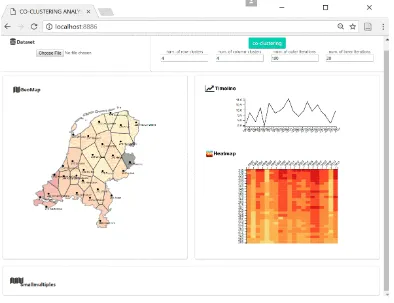
Figure 1 shows our web-based interactive platform where the spatio-temporal data is analyzed using BBAC_I and visualized using multiple linked visualizations. The platform, developed using Data-Driven Documents (D3, https://d3js.org/) and Open Web Standards, consists of both client- and server-side code. It is a graphical user interface (GUI) that allows users to load datasets, choose parameters for the clustering analysis and
subsequently presents the results in multiple linked visualizations. The client side runs inside any modern browser and makes use of D3.js for drawing visualizations. The server side of the application is implemented in R as it allows for convenient integration with existing R libraries (and thus fast implementation of additional clustering algorithms). The server will process the data received from the client, analyze it with the BBAC_I algorithm and return the results to the user’s browser for subsequent visualization and exploration. The jug library (https://cran.r-project.org/web/packages/jug/index.html) is used to set up a simple REST API in R that accepts POST requests with the BBAC_I parameters and the dataset as payload and will send back the co-clustering results. The BBAC_I algorithm, originally written in MATLAB, was ported to R by Felip Yanez (https://github.com/fnyanez/bbac) and subsequently adapted by the authors.
The graphical user interface in the client side contains five main parts from left to right and from top to bottom:
(1) Dataset. This part is to let users select their own data to be visualized and analyzed. By default, we use a dataset containing average yearly temperature from the Royal Netherlands Meteorological Institute (cf. section 3).
(2) Co-clustering and related parameters. This part is to let users select necessary input parameters for BBAC_I based on their own dataset, e.g. numbers of row- and column- clusters. When the co-clustering button is clicked, the client will request the R server to perform a co-clustering analysis of the current dataset with the filled parameters.
(3) GeoMap. This part is to visualize the spatial aspect of the dataset using a geographical map. The map is coloured using average values along all timestamps.
(4) Timeline and Heatmap. This part is to visualize the non-spatial aspects of the raw dataset or the co-clustering results. In its default view, the timeline shows the temporal distribution of the attribute values over all timestamps averaged along all locations in the dataset. As the timeline is linked with the GeoMap, it will update its display and show the temporal distribution of the attribute in the specific location that is chosen in the GeoMap. The heatmap provides a straightforward view of the dataset. It represents timestamps on the x-axis and locations on the y-axis. It then uses colour for each element to provide a straightforward view of each individual value in the dataset. Detailed information is exposed when the user hovers over an element.
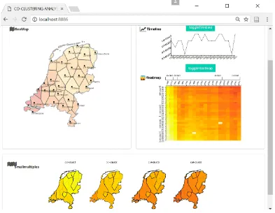
Once co-clustering is performed (see Figure 2), the timeline will update to display the temporal distribution of all timestamp-clusters by indicating the membership of each timestamp chronologically. The heatmap is used to visualize the location-clusters, timestamp-clusters as well as the location-timestamp co-clusters in the co-clustering results. The users can switch the view between the visualization of non-spatial aspects of the original dataset and the co-clustering results by using toggle buttons for the timeline and the heatmap respectively.
(5) Small multiples. The spatial distribution of co-clusters is visualized through a set of map-based small multiples for each of timestamp-clusters in the co-clustering results. Each individual map in this section is used to visualize the co-clusters for a single timestamp-cluster.
As such, the platform allows users to explore any dataset using co-clustering analysis. Users can select and upload their own dataset (as .csv file). The heatmap, timeline and geomap will update to display the user’s data. The user uses these visualizations to gain a better understanding of the dataset at hand and then choose appropriate parameters for the co-clustering analysis based on the specific objective of the analysis. Once the co-clustering analysis is finished, the corresponding results will be displayed in the platform’s graphs. The user can explore and interact with the results through the interactive, linked visualizations to assess the clustering results. They can toggle back to the visualization of the original dataset for comparison with the help of the toggle buttons. Importantly, the user can easily choose different sets of clustering parameters and instantly visualize those results. This is a great advantage over the more conventional ‘ad hoc’ approach to clustering where a user will execute a clustering algorithm with specific parameters and then create a set of visualizations by hand. If the analysis needs to be repeated with different parameters, the whole process needs to be repeated. As such, the platform allows for much faster, iterative and exploratory analysis through trial-and-error.
3. CASE STUDY DATASET
To illustrate the use of this web-based platform, we use yearly average temperature data collected from 28 weather stations in
the Netherlands from 1992 to 2011 (i.e. over 20 years). This dataset is freely available from the website of the Royal Netherlands Meteorological Institute, KNMI (https://data.knmi.nl/portal/KNMI-DataCentre.html)
.
Even though the Netherlands has a relatively small territory (41,500 km2), the unique location of this country (the west and north border the North Sea while the south and the east are bordered with Belgium and Germany, respectively), makes its weather influenced by both maritime (in the southwest) and continental (in the northeast) climates. Temperatures in the southwest are thus different from those in the northeast.
4. RESULTS
4.1 Visualizing the original dataset
As shown in Figure 1, when the Dutch yearly temperature dataset is selected, a Thiessen polygon map created based on the geographical coordinates of all the stations (also available on KNMI website) is used to show the spatial coverage of each station. In the Thiessen polygon map, each polygon is labelled by the station ID (e.g. 290) and its name (e.g. Twente). The coloured map where red indicates high temperature values shows the trend of decreasing temperature from southwest to northeast of the Netherlands.
The linear timeline shows the temporal distribution of the temperature of Dutch weather station (e.g. Twenthe in Figure 1) from 1992 to 2011. The timeline clearly shows the lowest temperature falls in 1996 and 2010, with 1993 following, while the highest temperature falls in recent years, e.g. 2006 and 2007. Although subtle, the slope of the timeline is positive with increasing temperature, which might due to global warming. By clicking other stations on the map, the temporal distributions of individual Dutch weather stations all indicate the similar trend. The heatmap offers the most straightforward view of the dataset using colours where red indicates high temperatures. It clearly shows in years 1996 and 2010, all weather stations have low temperatures. Year 1993 also has low temperatures but different with that in 1996 and 2010. By arranging stations from northeast to southwest of the country, the heatmap shows the increasing temperature from the top to bottom. These trends displayed in the heatmap are supported by those in geomap and the timeline.
4.2 Visualization of the co-clustering results
Based on previous work by Wu, Zurita-Milla et al. (2015) who used the same dataset for co-clustering analysis, the number of row and column clusters is set to 4. We also set 100 as the number of outer iterations and 20 as the number of inner iterations to guarantee the optimal results of BBAC_I. Once the ‘co -clustering’ button is clicked, these parameters are sent to the server together with the annual temperature dataset and processed by an R implementation of the BBAC_I routine. This takes about a second on a modern laptop. The co-clustering results are returned back to the user’s browsers to be automatically visualized using the heatmap, timeline and the small multiples as discussed before (Figure 2).
The heatmap in Figure 2 displays the 4 station-clusters, 4 year-clusters and their intersection as 4x4 station-year co-year-clusters. There are 2 x-axes and y-axes in the heatmap to indicate the membership of station- and year-clusters. The outer x- and y-axes are the year- and station- clusters from 1 to 4, with increasing temperature values. The inner x- and y-axes are years and stations, arranged according to the year- and station-cluster that
each belong to, to indicate their cluster membership. The intersection of each year- and station-cluster is one co-cluster, which contains similar temperature values along stations and years within that co-cluster. It is important to note here that the axes are no longer ordered chronologically and spatially but are ordered in such a way that the co-clusters have increasing temperature values from the left to right and from bottom to top of the heatmap. As such, the heatmap provides a clear understanding of station-clusters, year-clusters, co-clusters as well as their individual elements in the co-clustering results. With the toggle button named “toggleHeatmap”, the users can toggle back to the visualization of the raw dataset to have a comparison. With the arrangement of the x-axis from 1992 to 2011, the timeline is now used to visualize the temporal distribution of year-clusters and their elements in a chronological way. These year-clusters in the co-clustering results are supported by what we already inferred from the in the raw dataset: 1996 and 2010 in year-cluster1 with the lowest temperature values, 1993 alone in year-cluster2 and other recent years belonging to year-clusters with high temperature values. Again, with the toggle button named “toggleTimeline”, the user can toggle back to the original dataset for comparison.
The small multiples display station-clusters for each of 4 year-clusters. Within each individual map, the 4 regions with the thick outline correspond to the 4 station-clusters and each region is thus a station-year co-cluster in the heatmap. From northeast to southwest of the Netherlands and from cluster1 to year-cluster4, those co-clusters reveal the same trends of increasing temperature values as that in the heatmap. As such, our web-based platform helps the exploration of spatio-temporal patterns in the Dutch yearly temperature dataset using BBAC_I and also facilitates the understanding of the co-clustering results using these visualizations.
5. CONCLUSION
In this study, we presented an interactive web-based platform that enables co-clustering analysis of spatio-temporal data and subsequently facilitates the understanding and interpretation of the co-clustering results through multiple, interactive and linked visualizations. Specifically, we utilized the Bregman block average co-clustering algorithm with I-divergence (BBAC_I), which allows for the analysis of spatial and temporal patterns in a dataset simultaneously. In addition, we developed an interactive web-based platform with multiple linked visualizations to facilitate such analysis. As shown above, this platform allows users to upload their own dataset and display the dataset using multiple linked visualizations, which reveal different aspects of the dataset. The user can interact with these visualizations to obtain better understanding of their dataset, which helps them to select appropriate parameters for the co-clustering analysis. After the clustering analysis, users can directly view the co-clustering results from different angles using multiple visualizations. Users are also able to quickly change BBAC_I parameters and rerun co-clustering analysis if the results are not satisfactory. Designed as an iterative process, such co-clustering analysis can be repeated until users are satisfied with the results. In summary, while the use of BBAC_I enables the concurrent analysis of spatio-temporal patterns, the integration of such algorithms in an interactive web-based platform with multiple linked visualizations facilitates a deeper understanding and further interpretation of the co-clustering results.
be extended to the heatmap. In this way, when a station is clicked in the geomap, the timeline will change accordingly and the corresponding records in the heatmap will also be highlighted. Second, this functionality can also be extended to the visualization of co-clustering. The small multiples, timeline and geomap can be linked during the results phase as well. For example, if a user is interested in a specific co-cluster (e.g. station-cluster3/year-cluster2), they can click on the co-cluster to highlight it in the heatmap. It will then also highlight the corresponding co-cluster within both the small multiples and the timeline. Third, the functionality can be expanded by allowing users to use their own spatial point or polygon datasets. Currently a user can upload their own attribute dataset but not yet their own spatial point or polygon definition. This means that practical use is limited to Dutch point datasets. In the next version, users can upload their own map data in geojson format, either as point or polygon data. This will enable clustering analysis to be applied a wider range of datasets and geographic contexts. Fourth, we would like to allow users to set both their own color scheme as well as define their own class breaks. Currently the color scheme and class breaks are predefined for the temperature dataset. In the next version, users will be encouraged to select their own color scheme and pick appropriate class breaks based on their dataset and objectives of their analysis. Fifth, the present platform has only one single algorithm for co-clustering analysis (BBAC_I). Although interesting patterns can be revealed, different datasets and analytical objectives require more clustering algorithms. Thus, in the next version, we plan to add co-clustering algorithms (e.g. minimum sum-squared residue co-clustering algorithm) or one-way clustering algorithms (e.g. self-organizing maps (SOMs). Finally, the platform can then be released as a stand-alone website and the underlying client and server-side code can be made available as open-source.
REFERENCES
Deng, M., Q. Liu, J. Wang and Y. Shi (2013). "A general method of spatio-temporal clustering analysis." Science China Information Sciences 56(10): 1-14.
Kraak, M.-J. (2003). "Geovisualization illustrated." ISPRS Journal of Photogrammetry and Remote Sensing 57(5–6): 390-399.
O’Reilly, T. (2006). Web 2.0 compact definition: Trying again. Roth, R. E., D. Hart, R. Mead and C. Quinn (2017). "Wireframing for interactive & web-based geographic visualization: designing the NOAA Lake Level Viewer." Cartography and Geographic Information Science 44(4): 338-357.
Veenendaal, B. (2015). "Developing a map use model for web mapping and GIS." The International Archives of Photogrammetry, Remote Sensing and Spatial Information Sciences 40(4): 31.
Wu, X., R. Zurita-Milla and M. J. Kraak (2015). "Co-clustering geo-referenced time series: exploring spatio-temporal patterns in Dutch temperature data." International Journal of Geographical Information Science 29(4): 624-642.
Wu, X., R. Zurita‐Milla and M. J. Kraak (2016). "A novel analysis of spring phenological patterns over Europe based on co‐ clustering." Journal of Geophysical Research: Biogeosciences 121(6): 1434-1448.