Ordinary and Partial Differential Equation Routines in C, C , Fortran, Java, Maple, and MATLAB

(1)

(2)

(3)

(4)

CHAPMAN & HALL/CRC

A CRC Press Company

Boca Raton London New York Washington, D.C.

Ordinary and Partial Differential

Equation Routines in C, C++,

Fortran, Java

®

_{, Maple}

®

_{, and M}

ATLAB

®

(5)

MATLAB is a registered trademark of The MathWorks, Inc. For product information, please contact: The MathWorks, Inc.

3 Apple Hill Drive Natick, MA 01760-2098 Tel.: 508-647-7000 Fax: 508-647-7001 e-mail: info@mathworks.com

Web: www.mathworks.com http://www.mathworks.com/

This book contains information obtained from authentic and highly regarded sources. Reprinted material is quoted with permission, and sources are indicated. A wide variety of references are listed. Reasonable efforts have been made to publish reliable data and information, but the author and the publisher cannot assume responsibility for the validity of all materials or for the consequences of their use.

Neither this book nor any part may be reproduced or transmitted in any form or by any means, electronic or mechanical, including photocopying, microfilming, and recording, or by any information storage or retrieval system, without prior permission in writing from the publisher.

The consent of CRC Press LLC does not extend to copying for general distribution, for promotion, for creating new works, or for resale. Specific permission must be obtained in writing from CRC Press LLC for such copying.

Direct all inquiries to CRC Press LLC, 2000 N.W. Corporate Blvd., Boca Raton, Florida 33431. Trademark Notice: Product or corporate names may be trademarks or registered trademarks, and are used only for identification and explanation, without intent to infringe.

Visit the CRC Press Web site at www.crcpress.com

Library of Congress Card Number 2003055809 Printed in the United States of America 1 2 3 4 5 6 7 8 9 0

Printed on acid-free paper

Library of Congress Cataloging-in-Publication Data

Lee, H. J. (Hyun Jin)

Ordinary and partial differential equation routines in C, C++, Fortran, Java, Maple, and MATLAB / H.J. Lee and W.E. Schiesser.

p. cm.

Includes bibliographical references and index. ISBN 1-58488-423-1 (alk. paper)

1. Differential equations—Data processing. 2. Differential equations, Partial—Data processing. I. Schiesser, W. E. II. Title.

QA371.5.D37L44 2003

(6)

Initial value ordinary differential equations (ODEs) and partial differential equations (PDEs) are among the most widely used forms of mathematics in science and engineering. However, insights from ODE/PDE-based models are realized only when solutions to the equations are produced with accept-able accuracy and with reasonaccept-able effort.

Most ODE/PDE models are complicated enough (e.g., sets of simultane-ous nonlinear equations) to preclude analytical methods of solution; instead, numerical methods must be used, which is the central topic of this book.

The calculation of a numerical solution usually requires that well-established numerical integration algorithms are implemented in quality li-brary routines. The lili-brary routines in turn can be coded (programmed) in a variety of programming languages. Typically, for a scientist or engineer with an ODE/PDE- based mathematical model, finding routines written in a famil-iar language can be a demanding requirement, and perhaps even impossible (if such routines do not exist).

The purpose of this book, therefore, is to provide a set of ODE/PDE in-tegration routines written in six widely accepted and used languages. Our intention is to facilitate ODE/PDE-based analysis by using the library rou-tines to compute reliable numerical solutions to the ODE/PDE system of interest.

However, the integration of ODE/PDEs is a large subject, and to keep this discussion to reasonable length, we have limited the selection of algorithms and the associated routines. Specifically, we concentrate on explicit (nonstiff) Runge Kutta (RK) embedded pairs. Within this setting, we have provided integrators that are both fixed step and variable step; the latter accept a user-specified error tolerance and attempt to compute a solution to this required accuracy. The discussion of ODE integration includes truncation error moni-toring and control, h and p refinement, stability and stiffness, and explicit and implicit algorithms. Extensions to stiff systems are also discussed and illus-trated through an ODE application; however, a detailed presentation of stiff (implicit) algorithms and associated software in six languages was judged impractical for a book of reasonable length.

(7)

tools for the convenient solution of ODE/PDE models when programming in any of the six languages. The discussion is introductory with limited math-ematical details. Rather, we rely on numerical results to illustrate some basic mathematical properties, and we avoid detailed mathematical analysis (e.g., theorems and proofs), which may not really provide much assistance in the actual calculation of numerical solutions to ODE/PDE problems.

Instead, we have attempted to provide useful computational tools in the form of software. The use of the software is illustrated through a small number of ODE/PDE applications; in each case, the complete code is first presented, and then its components are discussed in detail, with particular reference to the concepts of integration, e.g., stability, error monitoring, and control. Since the algorithms and the associated software have limitations (as do all algorithms and software), we have tried to point out these limitations, and make suggestions for additional methods that could be effective.

Also, we have intentionally avoided using features specific to a particular language, e.g., sparse utilities, object-oriented programming. Rather, we have emphasized the commonality of the programming in the six languages, and thereby illustrate how scientific computation can be done in any of the lan-guages. Of course, language-specific features can be added to the source code that is provided.

We hope this format will allow the reader to understand the basic elements of ODE/PDE integration, and then proceed expeditiously to a numerical solu-tion of the ODE/PDE system of interest. The applicasolu-tions discussed in detail, two in ODEs and two in PDEs, can be used as a starting point (i.e., as tem-plates) for the development of a spectrum of new applications.

We welcome comments and questions about how we might be of assis-tance (directed to wes1@lehigh.edu). Information for acquiring (gratis) all the source code in this book is available from http://www.lehigh.edu/˜ wes1/ wes1.html. Additional information about the book and software is available from the CRC Press Web site, http://www.crcpress.com.

Dr. Fred Chapman provided expert assistance with the Maple program-ming. We note with sadness the passing of Jaeson Lee, father of H. J. Lee, during the completion of H. J. Lee’s graduate studies at Lehigh University.

(8)

1 Some Basics of ODE Integration. . . .1

1.1 General Initial Value ODE Problem. . . .1

1.2 Origin of ODE Integrators in the Taylor Series. . . .7

1.3 The Runge Kutta Method. . . .13

1.4 Accuracy of RK Methods. . . .18

1.5 Embedded RK Algorithms. . . .51

1.6 Library ODE Integrators. . . .72

1.7 Stability of RK Methods. . . .95

2 Solution of a 1x1 ODE System. . . .107

2.1 Programming in MATLAB. . . .107

2.2 Programming in C. . . .143

2.3 Programming in C++. . . .174

2.4 Programming in Fortran. . . .206

2.5 Programming in Java. . . .232

2.6 Programming in Maple. . . .263

3 Solution of a 2x2 ODE System. . . .291

4 Solution of a Linear PDE. . . .339

5 Solution of a Nonlinear PDE. . . .397

(9)

Appendix A Embedded Runge Kutta Pairs. . . .451

Appendix B Integrals from ODEs. . . .459

Appendix C Stiff ODE Integration. . . .465

C.1 The BDF Formulas Applied to the 2x2 ODE System. . . .465

C.2 MATLAB Program for the Solution of the 2x2 ODE System. . . .468

C.3 MATLAB Program for the Solution of the 2x2 ODE System Usingode23sandode15s . . . .477

Appendix D Alternative Forms of ODEs. . . .489

Appendix E Spatial p Refinement. . . .493

Appendix F Testing ODE/PDE Codes. . . .503

(10)

1

Some Basics of ODE Integration

The central topic of this book is the programming and use of a set of li-brary routines for the numerical solution (integration) of systems of initial value ordinary differential equations (ODEs). We start by reviewing some of the basic concepts of ODEs, including methods of integration, that are the mathematical foundation for an understanding of the ODE integration routines.

1.1 General Initial Value ODE Problem

The general problem for a single initial-value ODE is simply stated as

dy

dt = f(y, t), y(t0)=y0 (1.1)(1.2)

where

y= dependent variable

t= independent variable

f(y, t)= derivative function

t0= initial value of the independent variable

y0= initial value of the dependent variable

Equations 1.1 and 1.2 will be termed a 1x1 problem (one equation in one

un-known). The solution of this 1x1 problem is thedependent variable as a function

of the independent variable,y(t)(this function when substituted into Equations 1.1 and 1.2 satisfies these equations). This solution may be a mathematical

function, termed ananalytical solution.

(11)

To illustrate these ideas, we consider the 1x1 problem, from Braun1_(which will be discussed subsequently in more detail)

dy dt =λe

−αt_y, _y₍_t

0)=y0 (1.3)(1.4)

whereλandαare positive constants.

Equation 1.3 is termed afirst-order, linear, ordinary differential equation with

variable coefficients. These terms are explained below.

Term Explanation

Differential equation Equation 1.3 has a derivativedy/dt= f(y, t)₌λe−αt_y

Ordinary Equation 1.3 has only one independent variable,t, so that

the derivativedy/dtis atotalorordinaryderivative

First-order The highest-order derivative is first order (dy/dtis

first order)

Linear yand its derivativedy/dtare to the first power; thus,

Equation 1.3 is also termedfirst degree(do not confuse

orderanddegree)

Variable coefficient The coefficiente−αt_{is a function of the independent}

variable,t(if it were a function of the dependent

variable,y, Equation 1.3 would benonlinearor not

first degree)

The analytical solution to Equations 1.3 and 1.4 is from Braun:1

y(t)₌y0exp _λ

α(1−exp(−αt))

, y(0)₌y0 (1.5)

where exp(x)=ex_{. Equation 1.5 is easily verified as the solution to Equations}

1.3 and 1.4 by substitution in these equations:

Terms in Substitution of Equation 1.5 Equations 1.3 and 1.4 in Equations 1.3 and 1.4

dy

(12)

As an example of anxnproblem (nODEs inn unknowns), we will also

subsequently consider in detail the 2x2 system

dy1

dt =a11y1+a12y2 y1(0)=y10 dy2

dt =a21y1+a22y2 y2(0)=y20

(1.6)

The solution to Equations 1.6 is again the dependent variables,y1, y2, as a

function of the independent variable,t. Since Equations 1.6 arelinear, constant

coefficient ODEs, their solution is easily derived, e.g., by assuming exponential

functions intor by the Laplace transform. If we assume exponential functions

y1(t)=c1eλt y2(t)=c2eλt

(1.7)

wherec1,c2, andλare constants to be determined, substitution of Equations

1.7 in Equations 1.6 gives

c1λeλt =a11c1eλt+a12c2eλt c2λeλt =a21c1eλt+a22c2eλt

Cancellation ofeλt _{gives a system of algebraic equations (this is the reason}

assuming exponential solutions works in the case of linear, constant coefficient ODEs)

Equations 1.8 are the 2x2 case of thelinear algebraic eigenvalue problem

(13)

c=

The preceding matrices and vectors are

A nxncoefficient matrix

I nxnidentity matrix

c nx1 solution vector

0 nx1 zero vector

The reader should confirm that the matrices and vectors in Equation 1.9 have the correct dimensions for all of the indicated operations (e.g., matrix addi-tions, matrix-vector multiples).

Note that Equation 1.9 is alinear, homogeneous algebraic system

(homoge-neous means that the right-hand side (RHS) is the zero vector). Thus, Equation

1.9, or its 2x2 counterpart, Equations 1.8,will have nontrivial solutions (c=0)

if and only if (iff) the determinant of the coefficient matrix is zero, i.e.,

|A−λI| =0 (1.10)

Equation 1.10 is thecharacteristic equation for Equation 1.9 (note that it is a

scalar equation). The values ofλthat satisfy Equation 1.10 are theeigenvalues

of Equation 1.9. For the 2x2 problem of Equations 1.8, Equation 1.10 is

a11−λ a12 a21 a22−λ =0 or

(a11−λ)(a22−λ)−a21a12=0 (1.11)

Equation 1.11 is the characteristic equation or characteristic polynomial for

Equations 1.8; note that since Equations 1.8 are a 2x2 linear homogeneous

(14)

polynomial. Similarly, since Equation 1.9 is anxnlinear homogeneous

alge-braic system, its characteristic equation is anth-order polynomial.

Equation 1.11 can be factored by the quadratic formula

λ2−(a11+a22)λ+a11a22−a21a12=0

λ₁,λ₂₌ (a11+a22)±

(a11+a22)2−4(a11a22−a21a12)

2 (1.12)

Thus, as expected, the 2x2 system of Equations 1.8 has two eigenvalues.

In general, the nxn algebraic system, Equation 1.9, will have n

eigenval-ues, λ₁,λ₂,. . .,λn (which may be real or complex conjugates, distinct or repeated).

Since Equations 1.6 are linear constant coefficient ODEs, their general so-lution will be a linear combination of exponential functions, one for each eigenvalue

y1=c11eλ1t+c12eλ2t y2=c21eλ1t+c22eλ2t

(1.13)

Equations 1.13 have four constants which occur in pairs, one pair for each

eigenvalue. Thus, the pair [c11c21]T is theeigenvectorfor eigenvalueλ1while

[c12 c22]T is the eigenvector for eigenvalueλ2. In general, thenxnsystem of

Equation 1.9 will have anx1 eigenvector for each of itsneigenvalues. Note

that the naming convention for any constant in an eigenvector, ci j, is the

ith constant for the jth eigenvalue. We can restate the two eigenvectors for

Equation 1.13 (or Equations 1.8) as

Finally, the four constants in eigenvectors (Equations 1.14) are related through the initial conditions of Equations 1.6 and either of Equations 1.8

y10=c11eλ10+c12eλ20 y20=c21eλ10+c22eλ20

(1.15)

To simplify the analysis somewhat, we consider the special casea11=a22 =

−a , a21 =a12=b, whereaandbare constants. Then from Equation 1.12,

λ₁,λ₂₌ −2a±

(2a)2₋₄₍_a2₋_b2₎

(15)

From the first of Equations 1.8 forλ₌λ₁

(a11−λ1)c11+a12c21=0

or

(−a+(a−b))c11+bc21=0 c11=c21

Similarly, forλ₌λ₂

(a11−λ2)c12+a12c22 =0

or

(₋a+(a+b))c12+bc22 =0 c12 = −c22

Substitution of these results in Equations 1.15 gives

y10=c11−c22 y20=c11+c22

or

c11=

y10+y20

2 =c21

c22 =

y20−y10

2 = −c12

Finally, the solution from Equations 1.13 is

y1=

y10+y20

2 e

λ1t₋ y20−y10

2 e

λ2t

y2=

y10+y20

2 e

λ1t₊ y20−y10

2 e

λ2t

(1.17)

(16)

dy1

For the initial conditions of Equations 1.6

y10=

The ODE problems of Equations 1.3, 1.4, and 1.6 along with their analytical solutions, Equations 1.5 and 1.17, will be used subsequently to demonstrate the use of the ODE integration routines and to evaluate the computed

solu-tions. Since these problems are quite modest (1x1 and 2x2, respectively), we

will also subsequently consider two problems with substantially more ODEs. At the same time, these ODE systems will be considered as approximations to partial differential equations (PDEs); in other words, we will use systems of ODEs for the solution of PDEs.

1.2 Origin of ODE Integrators in the Taylor Series

In contrast to the analytical solutions presented previously (Equations 1.5 and 1.17), the numerical solutions we will compute are ordered pairs of numbers.

For example, in the case of Equation 1.3, we start from the pair(t0, y0)(the

initial condition of Equation 1.3) and proceed to compute paired values(ti, yi)

(17)

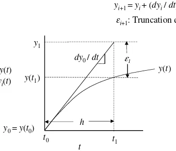
y(t): Exact solution

Stepping formula for the Euler method:

e

i+1: Truncation error

e 1

FIGURE 1.1

Stepping along the solution with Euler’s method.

The numerical integration is then a step-by-step algorithm going from the solution point(ti, yi)to the point(ti+1, yi+1).

This stepping procedure is illustrated in Figure 1.1 and can be represented mathematically by a Taylor series:

yi+1=yi+

and use this approximation to step along the solution from y0 to y1 (with

i =0), then fromy1toy2(withi =1), etc. This is the famousEuler’s method.

This stepping procedure is illustrated in Figure 1.1 (withi =0). Note that

Equation 1.19 is equivalent to projecting along a tangent line fromitoi+1. In

other words, we are representing the solution,y(t), by a linear approximation.

As indicated in Figure 1.1, an error,ε_i, will occur, which in the case of Figure

1.1 appears to be excessive. However, this apparently large error is only for

purposes of illustration in Figure 1.1. By taking a small enough step,h, the

error can, at least in principle, be reduced to any acceptable level. To see this,

consider the difference between the exact solution,y(ti+1), and the

approxi-mate solution,yi+1,ifhis halved in Figure 1.1 (note how the vertical difference

corresponding toεiis reduced). In fact, a major part of this book is devoted to

controlling the error,ε_i, to an acceptable level by varyingh.ε_i is termed the

(18)

Taylor series (Equation 1.18), in this case, to Equation 1.19. In other words,ε_i is the truncation error for Euler’s method, Equation 1.19.

We could logically argue that the truncation error could be reduced (for a

givenh) by including more terms in the Taylor, e.g., the second derivative

term(d2_y

i/dt2)(h2/2!). Although this is technically true, there is a practical

problem. For the general ODE, Equation 1.1, we have only the first derivative available

dyi

dt = f(yi, ti)

The question then in using the second derivative term of the Taylor series

is “How do we obtain the second derivative,d2_y

i/dt2?”. One answer would

be to differentiate the ODE, i.e.,

d2_y

Then we can substitute Equation 1.20 in Equation 1.18:

yi+1=yi+ fih+

where again subscript “i” means evaluated at pointi.

As an example of the application of Equation 1.21, consider the model ODE

dy

dt = f(y, t)=λy (1.22)

whereλis a constant. Then

fi =λyi

Equation 1.21 gives

yi+1=yi+λyih+λ (λyi) h2

2! =yi(1+λh+(λh)

2_/_2!₎

yi(1+λh+(λh)2/2!)is the Taylor series ofyieλhup to and including theh2term,

butyieλhis the analytical solution to Equation 1.22 with the initial condition

y(ti) = yi for the integration step,h =ti+1 −ti. Thus, as stated previously,

Equation 1.21 fits the Taylor series of the analytical solution to Equation 1.22

up to and including the(d2_y

i/dt2)(h2/2!)term.

(19)

derivative to arrive at the third derivative, etc. Clearly, however, the method quickly becomes cumbersome (and this is for only one ODE, Equation 1.1).

Application of thisTaylor series methodto systems of ODEs involves a lot of

differentiation. (Would we want to apply it to a system of 100 or 1000 ODEs? We think not.)

Ideally, we would like to have a higher-order ODE integration method (higher than the first-order Euler method) without having to take derivatives of the ODEs. Although this may seem like an impossibility, it can in fact be

done by theRunge Kutta (RK) method. In other words, theRK method can be

used to fit the numerical ODE solution exactly to an arbitrary number of terms in the underlying Taylor series without having to differentiate the ODE. We will investigate the RK method, which is the basis for the ODE integration routines described in this book.

The other important characteristic of a numerical integration algorithm (in addition to not having to differentiate the ODE) is a way of estimating the

truncation error,ε, so that the integration step,h, can be adjusted to achieve a

solution with a prescribed accuracy. This may also seem like an impossibility

since it would appear that in order to computeεwe need to know the exact

(analytical) solution. But if the exact solution is known, there would be no need to calculate the numerical solution. The answer to this apparent contradiction

is the fact that we will calculate anestimate of the truncation error(and not the

exact truncation error which would imply that we know the exact solution). To see how this might be done, consider computing a truncation error estimate for the Euler method. Again, we return to the Taylor series (which is the mathematical tool for most of the numerical analysis of ODE integration).

Now we will expand the first derivativedy/dt

dyi+1

i/dt2 is the second derivative we require in Equation 1.18. If the Taylor

series in Equation 1.23 is truncated after the h term, we can solve for this

second derivative

Equation 1.24 seems logical, i.e., the second derivative is afinite difference

(FD) approximationof the first derivative. Note that Equation 1.24 has the im-portant property that we can compute the second derivative without having to differentiate the ODE; rather, all we have to do is use the ODE twice, at

grid pointsiandi+1. Thus, the previous differentiation of Equation 1.20 is

(20)

become increasingly accurate with decreasinghsince the higher terms inhin Equation 1.23 (after the point of truncation) will become increasingly smaller.

Substituting Equation 1.24 in Equation 1.18 (truncated after theh2 _term)

gives

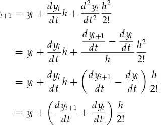
Equation 1.25 is the well-known modified Euler methodor extended Euler

method. We would logically expect that for a givenh, Equation 1.25 will give a more accurate numerical solution for the ODE than Equation 1.19. We will later demonstrate that this is so in terms of some ODE examples, and we will state more precisely how the truncation errors of Equations 1.19 and 1.25 vary

withh.

Note that Equation 1.25 uses the derivativedy/dtaveraged at pointsiand

i+1, as illustrated in Figure 1.2. Thus, whereas the derivative atiin Figure 1.1

+1: Truncation errors

FIGURE 1.2

(21)

is too large and causes the large overshoot of the numerical solution above

the exact solution (and thus, a relatively large value ofε_i), the averaging of

the derivatives ati andi +1 in Figure 1.2 reduces this overshoot (and the

truncation error is reduced fromε_iptoε_ic).

Equation 1.25 can be rearranged into a more useful form. If we assume

that the truncation error of Euler’s method,εi, is due mainly to the second

derivative term(d2_y

i/dt2)(h2/2!)of Equation 1.18 (which will be the case if

the higher-order terms in Equation 1.18 are negligibly small), then

ε_i₌ d

and Equation 1.25 can be written as a two-step algorithm:

y_ip₊₁= yi+

of Equation 1.26c are the same. While Equation 1.25 and Equations 1.26c are mathematically equivalent, Equations 1.26 have an advantage when used in

a computer program. Specifically, an algorithm that automatically adjustsh

to achieve a prescribed accuracy,tol, can be programmed in the following

steps:

1. Compute y_ip₊₁ by the Euler method, Equation 1.26a. The superscriptp

in this case denotes apredictedvalue.

2. Compute the estimated error, ε_i, from Equation 1.26b. Note that

dy_ip₊₁/dt= f(y_ip₊₁, ti+1), whereti+1 =ti+h.

3. Pose the question is εi<tol? If no, reduce h and return to 1. If yes,

continue to 4.

4. Add ε_i from 3 to y_ip₊₁ to obtain yc

i+1 according to Equation 1.26c. The

superscriptcdenotes acorrected value.

5. Incrementi,advancetitoti+1by addingh, go to 1. to take the next step

along the solution.

The algorithm of Equations 1.26 is termed apredictor-correctormethod, which

we will subsequently discuss in terms of a computer program.

To conclude this introductory discussion of integration algorithms, we

(22)

although they are not constant, but rather, vary along the solution) as

k1= f(yi, ti)h (1.27a)

k2= f(yi+k1, ti+h)h (1.27b)

the Euler method of Equation 1.19 can be written as (keep in minddy/dt=

f(y, t))

yi+1=yi+k1 (1.28)

and the modified Euler method of Equation 1.25 can be written

yi+1 =yi+ k1+k2

2 (1.29)

(the reader should confirm that Equation 1.25 and Equation 1.29 are the same). Also, the modified Euler method written in terms of an explicit error esti-mate, Equations 1.26, can be conveniently written in RK notation:

y_ip₊₁ =yi+k1 (1.30a)

ε_i ₌ (k2−k1)

2 (1.30b)

y_ic₊₁ =yi+k1+

(k2−k1)

2 =yi+

(k1+k2)

2 (1.30c)

However, the RK method is much more than just a convenient system of notation. As stated earlier, it is a method for fitting the underlying Taylor series of the ODE solution to any number of terms without having to differentiate

the ODE (it requires only the first derivative indy/dt= f(y, t)as we observe

in Equations 1.29 and 1.30). We next explore this important feature of the RK method, which is the mathematical foundation of the ODE integrators to be discussed subsequently.

1.3 The Runge Kutta Method

The RK method consists of a series of algorithms of increasing order.There

is only one first order RK method, the Euler method, which fits the underlying Taylor series of the solution up to and including the first derivative term, as indicated by Equation 1.19.

(23)

illustrated by the following development (based on the idea that the second-order RK method fits the Taylor series up to and including the second

deriva-tive term,(d2_y

i/dt2)(h2/2!)).

We start the analysis with a general RK stepping formula of the form

yi+1=yi+c1k1+c2k2 (1.31a)

wherek1andk2are RK “constants” of the form

k1= f(yi, ti)h (1.31b)

k2= f(yi+a2k1(yi, ti), ti+a2h)h= f(yi+a2f(yi, ti)h, ti+a2h)h (1.31c)

andc1, c2anda2are constants to be determined.

Ifk2from Equation 1.31c is expanded in a Taylor series in two variables,

k2 = f(yi+a2f(yi, ti)h, ti+a2h)h

=f(yi, ti)+ fy(yi, ti)a2f(yi, ti)h+ ft(yi, ti)a2h

h+O(h3) (1.32)

Substituting Equations 1.31b and 1.32 in Equation 1.31a gives

yi+1= yi+c1f(yi, ti)h+c2[f(yi, ti)+ fy(yi, ti)a2f(yi, ti)h

+ft(yi, ti)a2h]h+O(h3)

= yi+(c1+c2)f(yi, ti)h+c2[fy(yi, ti)a2f(yi, ti)

+ft(yi, ti)a2]h2+O(h3) (1.33)

Note that Equation 1.33 is a polynomial in increasing powers ofh; i.e., it has

the form of a Taylor series. Thus, if we expandyi+1in a Taylor series around

yi, we will obtain a polynomial of the same form, i.e., in increasing powers

ofh

merically. To match Equations 1.33 and 1.34, term-by-term (with like powers

ofh), we need to have [d f(yi, ti)/dt](h2/2!)in Equation 1.34 in the form of

fy(yi, ti)a2f(yi, ti)+ ft(yi, ti)a2in Equation 1.33.

If chain-rule differentiation is applied tod f(yi, ti)/dt

d f(yi, ti)

dt = fy(yi, ti) dyi

(24)

Substitution of Equation 1.35 in Equation 1.34 gives

yi+1=yi+ f(yi, ti)h+fy(yi, ti)f(yi, ti)+ ft(yi, ti) h2

2! +O(h

3₎ _(1.36)

We can now equate coefficients of like powers ofhin Equations 1.33 and 1.36

Power ofh Equation 1.33 Equation 1.36

h0 _y

Thus, we conclude

c1+c2 =1 c2a2 =1/2

(1.37)

This is a system of two equations in three unknowns or constants (c1, c2, a2);

thus, one constant can be selected arbitrarily (there are actually an infinite number of second-order RK methods, depending on the arbitrary choice of one of the constants in Equations 1.37). Here is one choice:

Choose c2=1/2

Other constants c1=1/2

a2=1

(1.38)

and the resulting second-order RK method is

yi+1 =yi+c1k1+c2k2=yi+ k1+k2

2 k1 = f(yi, ti)h

k2 = f(yi+a2k1(yi, ti), ti+a2h)h= f(yi+ f(yi, ti)h, ti+h)h which is the modified Euler method, Equations 1.27, 1.28, and 1.29.

For the choice

Choose c2=1

Other constants c1=0

a2=1/2

(1.39)

the resulting second-order RK method is

yi+1 =yi+c1k1+c2k2=yi+k2 (1.40a)

k1 = f(yi, ti)h (1.40b)

k2 = f(yi+a2k1(yi, ti), ti+a2h)h

= f(yi+(1/2)f(yi, ti)h, ti+(1/2)h)h

(25)

+1: Truncation error

FIGURE 1.3 Midpoint method.

which is themidpoint methodillustrated in Figure 1.3. As the name suggests, an

Euler step is used to compute a predicted value of the solution at the midpoint

between pointsi andi +1 according to Equation 1.40c. The corresponding

midpoint derivative (k2of Equation 1.40c) is then used to advance the solution

fromitoi+1 (according to Equation 1.40a).

Another choice of the constants in Equation 1.37 is (Iserles,2_{p. 84)}

Choose c2=3/4

(26)

equations and the final result (Iserles,2 _{p. 40). The third order stepping} for-mula is

yi+1=yi+c1k1+c2k2+c3k3 (1.43a)

The RK constants are

k1= f(yi, ti)h (1.43b)

k2= f(yi+a2k1, ti+a2h)h (1.43c)

k3= f(yi+b3k1+(a3−b3)k2, ti+a3h)h (1.43d)

Four algebraic equations define the six constantsc1, c2, c3, a2, a3, b3

(ob-tained by matching the stepping formula, Equation 1.43a, with the Taylor

series up to and including the term(d3_y

i/dt3)(h3/3!)

c1+c2+c3=1 (1.43e)

c2a2+c3a3=1/2 (1.43f)

c2a22+c3a32=1/3 (1.43g)

c3(a3−b3)a2=1/6 (1.43h)

To illustrate the use of Equations 1.43e to 1.43h, we can takec2 =c3 = 3₈,

and from Equation 1.43e,c1=1−3₈−3₈ = 2₈. From Equation 1.43f

(3/8)a2+(3/8)a3=1/2

ora2= 4₃−a3. From Equation 1.43g,

(3/8)(4/3−a3)2+(3/8)a32=1/3

ora3= 2₃(by the quadratic formula). Thus,a2= 4₃−2₃ = 2₃, and from Equation

1.43h,

(3/8)(2/3−b3)2/3=1/6

orb3=0.

This particular third-orderNystrom method(Iserles,2_{p. 40) is therefore}

yi+1=yi+(2/8)k1+(3/8)k2+(3/8)k3 (1.44a)

k1= f(yi, ti)h (1.44b)

k2= f(yi+(2/3)k1, ti+(2/3)h)h (1.44c)

k3= f(yi+(2/3)k2, ti+(2/3)h)h (1.44d)

(27)

The objective is to investigate the accuracy of these RK methods in computing solutions to an ODE test problem.

1.4 Accuracy of RK Methods

We start with the numerical solution of a single ODE, Equation 1.3, subject to initial condition Equation 1.4, by the Euler and modified Euler methods, Equation 1.28 and Equations 1.30. The analytical solution, Equation 1.5, can be used to calculate the exact errors in the numerical solutions.

Equation 1.3 models the growth of tumors, and this important application

is first described in the words of Braun1_{(the dependent variable in Equation}

1.3 is changed from “y” to “V” corresponding to Braun’s notation where V denotes tumor volume).

It has been observed experimentally that “free living” dividing cells, such as bacteria cells, grow at a rate proportional to the volume of the

dividing cells at that moment. LetV(t)denote the volume of the dividing

cells at timet. Then,

d V

dt =λV (1.45)

for some positive constantλ. The solution of Equation 1.45 is

V(t)₌V0eλ(t−t0) (1.46)

whereV0 is the volume of dividing cells at the initial timet0. Thus, free

living dividing cellsgrow exponentiallywith time. One important

conse-quence of Equation 1.46 is that the volume of the cells keeps doubling

every time interval of length ln 2/λ.

On the other hand, solid tumors do not grow exponentially with time. As the tumor becomes larger, the doubling time of the total tumor vol-ume continuously increases. Various researchers have shown that the data for many solid tumors is fitted remarkably well, over almost a 1000-fold increase in tumor volume, by the equation (previously Equation 1.5)

V(t)₌V0exp

λ

α(1−exp(−αt))

(1.47)

where exp(x)₌ex_{, and}_λ_and_α_{are positive constants.}

Equation 1.47 is usually referred to as aGompertzjanrelation. It says

that the tumor grows more and more slowly with the passage of time,

and that it ultimately approaches the limiting volume V0eλ/α. Medical

researchers have long been concerned with explaining this deviation from simple exponential growth. A great deal of insight into this problem can be

(28)

Equation 1.47 gives

(formerly Equation 1.3).

Two conflicting theories have been advanced for the dynamics of tumor growth. They correspond to the two arrangements

d V

of differential Equation 1.48. According to the first theory, the retarding effect of tumor growth is due to an increase in the mean generation time of the cells, without a change in the proportion of reproducing cells. As time goes on, the reproducing cells mature, or age, and thus divide more slowly. This theory corresponds to the bracketing of Equation 1.48a.

The bracketing of Equation 1.48b suggests the mean generation time of the dividing cells remains constant, and the retardation of growth is due to a loss in reproductive cells in the tumor. One possible

explana-tion for this is that anecrotic regiondevelops in the center of the tumor.

This necrosis appears at a critical size for a particular type of tumor, and thereafter, the necrotic “core” increases rapidly as the total tumor mass increases. According to this theory, a necrotic core develops because in many tumors the supply of blood, and thus of oxygen and nutrients, is al-most completely confined to the surface of the tumor and a short distance beneath it. As the tumor grows, the supply of oxygen to the central core by diffusion becomes more and more difficult, resulting in the formation of a necrotic core.

We can note the following interesting ideas about this problem:

• Equation 1.48 is a linear, variable coefficient ODE; it can also be

consid-ered to have a variable eigenvalue.

• The application of mathematical analysis to tumor dynamics apparently

started with a “solution” to an ODE, i.e., Equation 1.47.

• To gain improved insight into tumor dynamics, the question was posed

“Is there an ODE corresponding to Equation 1.47?”

• Once an ODE was found (Equation 1.48), it helped explain why the

solution, Equation 1.47, represents tumor dynamics so well.

• This is a reversal of the usual process of starting with a differential

equa-tion model, then using the soluequa-tion to explain the performance of the problem system.

(29)

%

% Program 1.1

% Tumor model of eqs. (1.47), (1.48) %

% Model parameters V0=1.0;

lambda=1.0; alpha=1.0; %

% Step through cases for ncase=1:4 %

% Integration step

if(ncase==1)h=1.0 ;nsteps=1 ;end

if(ncase==3)h=0.01 ;nsteps=100 ;end if(ncase==4)h=0.001;nsteps=1000;end %

% Variables for ODE integration tf=10.0;

t=0.0; %

% Initial condition V1=V0;

V2=V0; %

% Print heading

fprintf('\n\nh = %6.3f\n',h); fprintf(...

' t Ve V1 errV1 estV1

V2 errV2\n')

%

% Continue integration while t<0.999*tf %

% Take nsteps integration steps for i=1:nsteps

%

% Store solution at base point

V1b=V1; V2b=V2; tb=t; %

% RK constant k1

(30)

k12=lambda*exp(-alpha*t)*V2*h; %

% RK constant k2

V1=V1b+k11; V2=V2b+k12;

t=tb+h;

k22=lambda*exp(-alpha*t)*V2*h; %

% RK step

V2=V2b+(k12+k22)/2.0; t=tb+h;

end %

% Print solutions and errors

Ve=V0*exp((lambda/alpha)*(1.0-exp(-alpha*t))); errV1=V1-Ve;

errV2=V2-Ve; estV1=V2-V1;

fprintf('%5.1f%9.4f%9.4f%15.10f%15.10f%9.4f%15.10f\n',... t,Ve,V1,errV1,estV1,V2,errV2);

%

% Continue integration end

%

% Next case end

Program 1.1

MATLAB program for the integration of Equation 1.48 by the modified Euler method of Equations 1.28 and 1.30

We can note the following points about Program 1.1:

• The initial condition and the parameters of Equation 1.48 are first defined

(note that % defines a comment in MATLAB):

%

% Model parameters V0=1.0;

lambda=1.0; alpha=1.0;

• The program then steps through four cases corresponding to the

inte-gration stepsh=1.0,0.1,0.01,0.001:

%

(31)

%

% Integration step

if(ncase==3)h=0.01 ;nsteps=100 ;end if(ncase==4)h=0.001;nsteps=1000;end

For each h, the corresponding number of integration steps isnsteps.

Thus, the product (h)(nsteps) = 1 unit in t for each output from the

program; i.e., the output from the program is att=0,1,2,. . .,10.

• For each case, the initial and final values oftare defined, i.e.,t=0, t f =

10, and the initial condition,V(0)₌V0 is set to start the solution:

%

t=0.0; %

% Initial condition V1=V0;

V2=V0;

Two initial conditions are set, one for the Euler solution, computed as

V1, and one for the modified Euler solution,V2 (subsequently, we will

program the solution vector, in this case [V1V2]T, as a one-dimensional

(1D) array).

• A heading indicating the integration step, h, and the two numerical

solutions is then displayed. “. . .” indicates a line is to be continued on

the next line. (Note:. . .does not work in a character string delineated by

single quotes, so the character string in the secondfprintfstatement has

been placed on two lines in order to fit within the available page width; to execute this program, the character string should be returned to one line.)

%

% Print heading

' t Ve V1 errV1 estV1

V2 errV2\n')

• Awhileloop then computes the solution until the final time,t f, is reached:

%

(32)

Of course, at the beginning of the execution, t = 0 so thewhile loop continues.

• nstepsEuler and modified Euler steps are then taken:

%

V1b=V1; V2b=V2; tb=t;

At each point along the solution (pointi), the solution is stored for

sub-sequent use in the numerical integration.

• The first RK constant,k1, is then computed for each dependent variable

in [V1V2)]T _{according to Equation 1.27a:}

%

% RK constant k1

k11=lambda*exp(-alpha*t)*V1*h; k12=lambda*exp(-alpha*t)*V2*h;

Note that we have used the RHS of the ODE, Equation 1.48, in computing

k1.k11isk1forV1, andk12 isk1forV2. Subsequently, the RK constants

will be programmed as 1D arrays, e.g., [k1(1)k1(2)]T.

• The solution is then advanced from the base point according to Equation

1.28:

%

% RK constant k2

V1=V1b+k11; V2=V2b+k12;

t=tb+h;

k22=lambda*exp(-alpha*t)*V2*h;

The second RK constant,k2forV2, is then computed according to

Equa-tion 1.27b. At the same time, the independent variable,t, is advanced.

• The modified Euler solution,V2, is then computed according to Equation

1.29:

%

% RK step

V2=V2b+(k12+k22)/2.0; t=tb+h;

end

The advance of the independent variable,t, was done previously and is

(33)

for the modified Euler method. Theendstatement ends the loop ofnsteps steps, starting with

for i=1:nsteps

• The exact solution,Ve, is computed from Equation 1.47. The exact error

in the Euler solution,errV1, and in the modified Euler solution,errV2,

are then computed. Finally, the difference in the two solutions,estV1=

V2−V1, is computed as an estimate of the error inV1. The independent

variable,t, the two dependent variables, V1, V2, and the three errors,

errV1, errV2, estV1, are then displayed.

%

Ve=V0*exp((lambda/alpha)*(1.0-exp(-alpha*t))); errV1=V1-Ve;

errV2=V2-Ve; estV1=V2-V1;

fprintf('%5.1f%9.4f%9.4f%15.10f%15.10f%9.4f

%15.10f\n',...t,Ve,V1,errV1,estV1,V2,errV2);

The output from thefprintfstatement is considered subsequently.

• Thewhile loop is then terminated, followed by the end of theforloop

that setsncase:

%

% Next case end

We now consider the output from this program listed below (reformatted slightly to fit on a printed page):

h = 1.000

Euler method

t Ve V1 errV1 estV1

1.0 1.8816 2.0000 0.1184036125 -0.1321205588

2.0 2.3742 2.7358 0.3615489626 -0.3514091013

3.0 2.5863 3.1060 0.5197432882 -0.4929227741

4.0 2.6689 3.2606 0.5916944683 -0.5573912375

5.0 2.7000 3.3204 0.6203353910 -0.5830821148

6.0 2.7116 3.3427 0.6311833526 -0.5928173392

7.0 2.7158 3.3510 0.6352171850 -0.5964380611

(34)

9.0 2.7179 3.3552 0.6372559081 -0.5982681335

10.0 2.7182 3.3556 0.6374579380 -0.5984494919

modified Euler method

t Ve V2 errV2

1.0 1.8816 1.8679 -0.0137169464

2.0 2.3742 2.3843 0.0101398613

3.0 2.5863 2.6131 0.0268205142

4.0 2.6689 2.7033 0.0343032307

5.0 2.7000 2.7373 0.0372532762

6.0 2.7116 2.7499 0.0383660134

7.0 2.7158 2.7546 0.0387791239

8.0 2.7174 2.7563 0.0389316092

9.0 2.7179 2.7569 0.0389877746

10.0 2.7182 2.7572 0.0390084461

h = 0.100

Euler method

t Ve V1 errV1 estV1

1.0 1.8816 1.8994 0.0178364041 -0.0178773733

2.0 2.3742 2.4175 0.0433341041 -0.0430037365

3.0 2.5863 2.6438 0.0575343031 -0.0569959440

4.0 2.6689 2.7325 0.0635808894 -0.0629558472

5.0 2.7000 2.7660 0.0659265619 -0.0652682467

6.0 2.7116 2.7784 0.0668064211 -0.0661356782

7.0 2.7158 2.7829 0.0671324218 -0.0664570816

8.0 2.7174 2.7846 0.0672526658 -0.0665756310

9.0 2.7179 2.7852 0.0672969439 -0.0666192852

10.0 2.7182 2.7855 0.0673132386 -0.0666353503

t Ve V2 errV2

1.0 1.8816 1.8816 -0.0000409693

2.0 2.3742 2.3745 0.0003303677

3.0 2.5863 2.5868 0.0005383591

4.0 2.6689 2.6696 0.0006250422

5.0 2.7000 2.7007 0.0006583152

(35)

7.0 2.7158 2.7165 0.0006753402

8.0 2.7174 2.7180 0.0006770348

9.0 2.7179 2.7186 0.0006776587

10.0 2.7182 2.7188 0.0006778883

h = 0.010

Euler method

t Ve V1 errV1 estV1

1.0 1.8816 1.8835 0.0018696826 -0.0018697473

2.0 2.3742 2.3786 0.0044269942 -0.0044231149

3.0 2.5863 2.5921 0.0058291952 -0.0058231620

4.0 2.6689 2.6754 0.0064227494 -0.0064158254

5.0 2.7000 2.7067 0.0066525021 -0.0066452372

6.0 2.7116 2.7183 0.0067386119 -0.0067312197

7.0 2.7158 2.7226 0.0067705073 -0.0067630680

8.0 2.7174 2.7242 0.0067822704 -0.0067748139

9.0 2.7179 2.7247 0.0067866019 -0.0067791389

10.0 2.7182 2.7249 0.0067881959 -0.0067807306

t Ve V2 errV2

1.0 1.8816 1.8816 -0.0000000647

2.0 2.3742 2.3742 0.0000038793

3.0 2.5863 2.5863 0.0000060332

4.0 2.6689 2.6690 0.0000069239

5.0 2.7000 2.7000 0.0000072649

6.0 2.7116 2.7116 0.0000073922

7.0 2.7158 2.7158 0.0000074392

8.0 2.7174 2.7174 0.0000074566

9.0 2.7179 2.7180 0.0000074629

10.0 2.7182 2.7182 0.0000074653

h = 0.001

Euler method

t Ve V1 errV1 estV1

1.0 1.8816 1.8818 0.0001878608 -0.0001878611

(36)

3.0 2.5863 2.5868 0.0005836997 -0.0005836386

4.0 2.6689 2.6696 0.0006429444 -0.0006428744

5.0 2.7000 2.7007 0.0006658719 -0.0006657985

6.0 2.7116 2.7122 0.0006744643 -0.0006743896

7.0 2.7158 2.7165 0.0006776469 -0.0006775717

8.0 2.7174 2.7180 0.0006788206 -0.0006787453

9.0 2.7179 2.7186 0.0006792528 -0.0006791774

10.0 2.7182 2.7188 0.0006794118 -0.0006793364

t Ve V2 errV2

1.0 1.8816 1.8816 -0.0000000003

2.0 2.3742 2.3742 0.0000000394

3.0 2.5863 2.5863 0.0000000610

4.0 2.6689 2.6689 0.0000000700

5.0 2.7000 2.7000 0.0000000734

6.0 2.7116 2.7116 0.0000000747

7.0 2.7158 2.7158 0.0000000751

8.0 2.7174 2.7174 0.0000000753

9.0 2.7179 2.7179 0.0000000754

10.0 2.7182 2.7182 0.0000000754

We can note the following points about this output:

• Considering first the output for the Euler method att=1:

h Ve V1 errV1 estV1 V1 +estV1

1 1.8816 2.0000 0.1184036125 −0.1321205588 1.8679

0.1 1.8816 1.8994 0.0178364041 −0.0178773733 1.8815

0.01 1.8816 1.8835 0.0018696826 −0.0018697473 1.8816

0.001 1.8816 1.8818 0.0001878608 −0.0001878611 1.8816

We can note the following points for this output:

— The exact error,errV1, decreases linearly with integration step,h.

For example, whenhis decreased from 0.01 to 0.001,errV1 decreases

from 0.0018696826 to 0.0001878608. Roughly speaking, as the decimal

point inh moves one place, the decimal point inerrV1 moves one

place. However, this is true only when h becomes small (so that

higher-order terms in the underlying Taylor series become negligibly small).

— Thus, the error in the Euler method is proportional toh

(37)

whereCis a constant. The Euler method is therefore termedfirst order in horfirst order correctorof order h, which is usually designated as

errV1=O(h) where “O” denotes “of order.”

— The estimated error,estV1 is alsofirst order in h(note again, that ash

is decreased by a factor of 1/10,estV1 decreases by a factor of 1/10).

Furthermore, the estimated error,estV1, approaches the exact error,

errV1 for smallh. This is an important point since the estimated error

can be computed without knowing the exact solution; in other words, we canestimate the error in the numerical solution without knowing the exact solution. The estimated error,estV1=V2−V1 is the same asεigiven by Equation 1.26b and discussed in words following Equations 1.26.

— If the estimated error,estV1, is added as a correction to the

numeri-cal solution,V1, the corrected solution (in the last column) is much

closer to the exact solution,Ve. Thus, the estimated error can not only

be used to judge the accuracy of the numerical solution, and thereby

used to decrease h if necessary to meet a specified error tolerance

(see again Equation 1.26b and the subsequent discussion), but the

estimated error can beused as a correction for the numerical solution

to obtain a more accurate solution. We will make use of these impor-tant features of the estimated error in the subsequent routines that

automatically adjust the step,h, to achieve a specified accuracy.

• Considering next the output for the modified Euler method att=1:

h Ve V2 errV2

1 1.8816 1.8679 −0.0137169464

0.1 1.8816 1.8816 −0.0000409693

0.01 1.8816 1.8816 −0.0000000647

0.001 1.8816 1.8816 −0.0000000003

— The exact error for the modified Euler method,errV2, is substantially

smaller than the error for the Euler method,errV1 andestV1. This is

to be expected since the modified Euler method includes the second

derivative term in the Taylor series,(d2y/dt2)(h2/2!), while the Euler

method includes only the first derivative term,(dy/dt)(h/1!).

— In other words, the exact error,errV2, decreases much faster withh

than doeserrV1. The order of this decrease is difficult to assess from

the solution att =1. For example, whenhis decreased from 0.1 to

0.01, the number of zeros after the decimal point increases from four

(−0.000040969) to seven (−0.0000000647) (or roughly, a decrease of

(38)

after the decimal point only increases from seven (−0.0000000647) to

nine (−0.0000000003) (or roughly, a decrease of 1/100). Thus, is the

order of the modified Euler methodO(h2₎_or_O(h3₎_?

• We come to a somewhat different conclusion if we consider the modified

Euler solution att=10:

h Ve V2 errV2

1 2.7182 2.7572 0.0390084461

0.1 2.7182 2.7188 0.0006778883

0.01 2.7182 2.7182 0.0000074653

0.001 2.7182 2.7182 0.0000000754

— The error,errV2, now appears to besecond order. For example, whenh

is reduced from 0.1 to 0.01, the error decreases from 0.0006778883 to

0.0000074653, a decrease of approximately 1/100. Similarly, whenh

is reduced from 0.01 to 0.001, the error decreases from 0.0000074653

to 0.0000000754, again a decrease of approximately 1/100. Thus, we

can conclude that at least for this numerical output at t = 10, the

modified Euler method appears to be second order correct, i.e.,

errV2=O(h2)

We shall generally find this to be the case (the modified Euler method is second order), although, clearly, there can be exceptions (i.e., the

output att=1).

• Finally, we can come to some additional conclusions when comparing

the output for the Euler and modified Euler methods:

— Generally, for both methods, the accuracy of the numerical solutions

can be improved by decreasingh. This process is termedh refinement,

and is an important procedure in ODE library integration routines,

i.e., decreasinghto improve the solution accuracy.

— An error in the numerical solution, in this caseestV1, can be estimated

by subtracting the solutions from two methods of different orders,

i.e.,estV1=V2−V1. This estimated error can then be used to adjust

h to achieve a solution of prescribed accuracy (see Equations 1.26).

This procedure of subtracting solutions of different order is termed p refinementsince generally the order of the approximations is stated in terms of a variable “p”, i.e.,

error=O(hp)

In the present case, p = 1 for the Euler method (it is first order

correct), andp=2 for the modified Euler method (it is second order

(39)

we can estimate the error in the numerical solution (without having to know the exact solution), and thereby make some adjustments in

hto achieve a specified accuracy.

— The integration errors we have been considering are calledtruncation

errorssince they result from truncation of the underlying Taylor series

(after(dy/dt)(h/1!)and(d2_y/dt2_)(h2_/_2!₎_{for the Euler and modified}

Euler methods, respectively).

— The preceding analysis and conclusions are based on a sufficiently

small value ofhthat the higher-order terms (inh) in the Taylor series

(after the point of truncation) are negligibly small.

— We have not produced a rigorous proof ofO(h)andO(h2₎_{for the}

Eu-ler method and modified EuEu-ler method. Rather, all of the preceding analysis was through the use of a single, linear ODE, Equation 1.48.

Thus, we cannot conclude that these order conditions are generally

true (for any system of ODEs). Fortunately, they have been observed to be approximately correct for many ODE systems, both linear and nonlinear.

— Higher-order RK algorithms that fit more of the terms of the

underly-ing Taylor series are available (consider the third-order RK method of Equations 1.44). The preceding error analysis can be applied to them in the same way, and we will now consider again the results for the numerical solution of Equation 1.48. In other words, we can

considerhandprefinement for higher-order RK methods.

— The higher order of the modified Euler method, O(h2₎_{, relative to}

the Euler method, O(h), was achieved through additional

compu-tation. Specifically, in the preceding MATLAB program, the Euler

method required only onederivative evaluation(use of Equation 1.48)

for each step along the solution, while the modified Euler method re-quired two derivative evaluations for each step along the solution. In other words, we pay a “computational price” of additional derivative evaluations when using higher-order methods (that fit more of the underlying Taylor series). However, this additional computation is usually well worth doing (consider the substantially more accurate solution of Equation 1.48 when using the modified Euler method relative to the Euler method, and how much more quickly the

er-ror dropped off with decreasingh, i.e.,O(h2₎_vs._O(h)_{). Generally,}

an increase in the order of the method of one (e.g., O(h)to O(h2₎₎

requires one additional derivative evaluation for order up to and in-cluding four; beyond fourth order, increasing the order of accuracy by one will require more than one additional derivative evaluation (we shall observe this for a fifth-order RK method to be discussed subsequently).

— In all of the preceding discussion, we have assumed that the solution

(40)

Taylor series), which is basically a polynomial inh. Of course, this does not have to be the case, but we are assuming that in using

numerical ODE integration algorithms, for sufficiently smallh, the

Taylor series approximation of the solution is sufficiently accurate for the given ODE application.

— The RK method is particularly attractive since it can be formulated

for increasing orders (more terms in the Taylor series) without having to differentiate the differential equation to produce the higher-order derivatives required in the Taylor series. Thus, all we have to do in the programming of an ODE system is numerically evaluate the derivatives defined by the ODEs.

— As we shall see in subsequent examples, the RK method can be

ap-plied to thenxnproblem (nODEs inn unknowns) as easily as we

applied it to the 1x1 problem of Equation 1.48. Thus, it is a general

procedure for the solution of systems of ODEs of virtually any order

(nxn) and complexity (which is why it is so widely used). In other

words, the RK algorithms (as well as other well-established integra-tion algorithms) are a powerful tool in the use of ODEs in science and engineering; we shall see that the same is also true for PDEs.

We now conclude this section by considering the errors in the numerical

solution of Equation 1.48 with a(2,3)RK pair (i.e.,O(h2₎_and_O(h3₎_{in analogy}

with the(1,2)pair of the Euler and modified Euler methods), and then a(4,5)

pair (O(h4₎_and _O(h5₎_{). This error analysis will establish that the expected}

order conditions are realized and also will provide two higher RK pairs that we can then put into library ODE integration routines.

The(2,3)pair we considered previously (Equations 1.42 and 1.44) is coded

in the following program. Here we have switched back from the dependent

variableVused previously in Equation 1.48 to the more commonly usedyin

Equation 1.3. Also,y2 is the solution of Equation 1.3 using the second-order

RK of Equations 1.42 while y3 is the solution using the third-order RK of

Equations 1.44.

%

% Program 1.2

% Tumor model of eqs. (1.47), (1.48) % (or eqs. (1.3), (1.4), (1.5)) %

% Model parameters y0=1.0;

lambda=1.0; alpha=1.0; %

(41)

%

% Integration step

if(ncase==3)h=0.01 ;nsteps=100 ;end if(ncase==4)h=0.001;nsteps=1000;end %

t=0.0; %

% Initial condition y2=y0;

y3=y0; %

% Print heading

' t ye y2 erry2 esty2

y3 erry3\n')

%

% Continue integration while t<0.999*tf %

%

y2b=y2; y3b=y3; tb=t; %

% RK constant k1

k12=lambda*exp(-alpha*t)*y2*h; k13=lambda*exp(-alpha*t)*y3*h; %

% RK constant k2

y2=y2b+(2.0/3.0)*k12;

% RK integration K3

(42)

t=tb +(2.0/3.0)*h;

k33=lambda*exp(-alpha*t)*y3*h; %

% RK step

y2=y2b+(1.0/4.0)*k12+(3.0/4.0)*k22;

y3=y3b+(1.0/4.0)*k13+(3.0/8.0)*k23+(3.0/8.0)*k33; t=tb+h;

end %

ye=y0*exp((lambda/alpha)*(1.0-exp(-alpha*t))); erry2=y2-ye;

erry3=y3-ye; esty2=y3-y2;

fprintf('%5.1f%9.4f%9.4f%15.10f%15.10f%9.4f%15.10f\n',... t,ye,y2,erry2,esty2,y3,erry3);

%

% Next case end

Program 1.2

Program for the integration of Equation 1.48 by the RK(2,3)pair of Equations

1.42 and 1.44

Program 1.2 closely parallels Program 1.1. The only essential difference is

the coding of the RK(2,3)pair of Equations 1.42 and 1.44 in place of the RK

(1,2)pair of Equations 1.28 and 1.29. We can note the following points about

Program 1.2:

• Initial condition (Equation 1.4) is again set for y2 and y3 to start the

numerical solutions:

%

% Initial condition y2=y0;

y3=y0;

• The integration proceeds with the outer while loop (that eventually

reaches the final time, t f), and an innerforloop that takesnsteps RK

steps for each output. For each pass through the inner loop, the solution is stored at the base point for subsequent use in the RK formulas:

%

(43)

%

y2b=y2; y3b=y3; tb=t;

• The RK constantk1 is computed for each dependent variable by using

Equation 1.3 (k12 for thek1ofy2 andk13 for thek1ofy3):

%

% RK constant k1

k12=lambda*exp(-alpha*t)*y2*h; k13=lambda*exp(-alpha*t)*y3*h;

• The solution is then advanced from the base point using a 2

3 weighting

applied tok1andh(in accordance with Equations 1.42 and 1.44):

%

% RK constant k2

y2=y2b+(2.0/3.0)*k12; y3=y3b+(2.0/3.0)*k13;

t=tb +(2.0/3.0)*h;

k22=lambda*exp(-alpha*t)*y2*h; k23=lambda*exp(-alpha*t)*y3*h;

This advance of the dependent and independent variables sets the stage

for the calculation ofk2(again, using Equation 1.3).

• k3is computed fory3 (it is not required fory2):

%

% RK integration K3

y3=y3b+(2.0/3.0)*k23; t=tb +(2.0/3.0)*h;

k33=lambda*exp(-alpha*t)*y3*h;

• All the required RK constants have now been computed, and the

solu-tions can be advanced to the next point using the stepping formulas:

%

% RK step

y2=y2b+(1.0/4.0)*k12+(3.0/4.0)*k22;

y3=y3b+(1.0/4.0)*k13+(3.0/8.0)*k23+(3.0/8.0)*k33; t=tb+h;

end

Note that the stepping formula fory2 does not includek3. Theend

(44)

• The solutions,y2 andy3, and associated errors are then displayed:

%

ye=y0*exp((lambda/alpha)*(1.0-exp(-alpha*t))); erry2=y2-ye;

erry3=y3-ye; esty2=y3-y2;

fprintf('%5.1f%9.4f%9.4f%15.10f%15.10f%9.4f

%15.10f\n',...t,ye,y2,erry2,esty2,y3,erry3);

• Finally, thewhileloop is concluded, followed by theforloop that sets the

values ofh, and the initial and final values oft:

%

% Next case end

• Note that Equation 1.3 was used twice to computek1andk2fory2 (two

derivative evaluations), and Equation 1.3 was used three times to

com-putek1,k2, andk3fory3 (three derivative evaluations). This again

illus-trates the additional computation required, in this case, the calculation

of k3, to achieve higher-order results (O(h3)rather than O(h2)). This

improved accuracy is evident in the following output from Program 1.2.

The output from Program 1.2 is listed below (again, with some minor for-matting to fit on a printed page):

h = 1.000

Second order RK

t ye y2 erry2 esty2

1.0 1.8816 1.8918 0.0101750113 -0.0185221389

2.0 2.3742 2.3995 0.0252529307 -0.0352289432

3.0 2.5863 2.6170 0.0307095187 -0.0408693758

4.0 2.6689 2.7014 0.0324302424 -0.0425724266

5.0 2.7000 2.7330 0.0330043494 -0.0431262652

6.0 2.7116 2.7448 0.0332064307 -0.0433188969

7.0 2.7158 2.7491 0.0332794779 -0.0433881911

8.0 2.7174 2.7507 0.0333061722 -0.0434134670

9.0 2.7179 2.7513 0.0333159682 -0.0434227360

(45)

Third order RK

t ye y3 erry3

1.0 1.8816 1.8732 -0.0083471276

2.0 2.3742 2.3642 -0.0099760125

3.0 2.5863 2.5761 -0.0101598572

4.0 2.6689 2.6588 -0.0101421842

5.0 2.7000 2.6899 -0.0101219158

6.0 2.7116 2.7014 -0.0101124662

7.0 2.7158 2.7057 -0.0101087132

8.0 2.7174 2.7073 -0.0101072948

9.0 2.7179 2.7078 -0.0101067678

10.0 2.7182 2.7081 -0.0101065733

h = 0.100

Second order RK

t ye y2 erry2 esty2

1.0 1.8816 1.8819 0.0003179977 -0.0003270335

2.0 2.3742 2.3748 0.0005660244 -0.0005762943

3.0 2.5863 2.5869 0.0006477190 -0.0006581264

4.0 2.6689 2.6696 0.0006733478 -0.0006837363

5.0 2.7000 2.7007 0.0006819708 -0.0006923405

6.0 2.7116 2.7122 0.0006850226 -0.0006953838

7.0 2.7158 2.7165 0.0006861284 -0.0006964862

8.0 2.7174 2.7181 0.0006865329 -0.0006968894

9.0 2.7179 2.7186 0.0006866814 -0.0006970374

10.0 2.7182 2.7188 0.0006867360 -0.0006970918

Third order RK

t ye y3 erry3

1.0 1.8816 1.8816 -0.0000090358

2.0 2.3742 2.3742 -0.0000102699

3.0 2.5863 2.5862 -0.0000104074

4.0 2.6689 2.6689 -0.0000103885

5.0 2.7000 2.7000 -0.0000103698

6.0 2.7116 2.7115 -0.0000103611

7.0 2.7158 2.7158 -0.0000103577

8.0 2.7174 2.7174 -0.0000103564

9.0 2.7179 2.7179 -0.0000103560