APPLICATION OF CONDITIONAL PROBABILITY IN
PREDICTING INTERVAL PROBABILITY OF DATA
QUERYING
Rolly Intan
Faculty of Industrial Technology, Informatics Engineering Department, Petra Christian University
Email: [email protected]
ABSTRACT: This paper discusses fuzzification of crisp domain into fuzzy classes providing fuzzy domain. Relationship between two fuzzy domains,
X
i andX
j, can be represented by using a matrix,w
ij. IfX
i has n elements of fuzzy data andX
j has m elements of fuzzy data thenw
ij isn
×
m
matrix. Our primary goal in this paper is to generate some formulas for predicting interval probability in the relation to data querying, i.e., given John is 30 years old and he has MS degree, how about his probability to get high salary.Keywords: Fuzzy Conditional Probability Relation, Data Querying, Interval Probability, Mass Assignment, Point Semantic Unification.
1. INTRODUCTION
In a system, we will find that every component has relation one to each other. For example, system CAREER has some components such as education, age, and
salary in which we realize that all of them has interrelationship as in general higher education means higher salary, or older someone will get higher salary, or in a certain area, percentage of mid-40’s of persons who has doctoral degree is 30 percent, etc.
In this paper, we process a certain relational database by classifying every domain into several value of data or elements of the component, i.e., domain or component age can be classified into {about_20, about_25, …, about_60}. With assumption that every classified data is a fuzzy set, we must determine a member-ship function which represents degree of element belonging to the fuzzy set, i.e.,
about_30={0.2/26, 04/27, 0.6/28, 0.8/29, 1/30, 0.8/31, 0.6/32, 0.4/33, 0.2/34}. Next, we apply the all membership function into the previous relational database to find every membership value for every item data. And then, by using conditional probabilistic theory, we construct a model
to describe interrelationship among all components of the system. Relationship between two components, X1 and X2, of a system is expressed in a matrix
w
12. If component X1 has n elements, X2has melements then matrix
w
12 isn
×
m
matrix, wherea
12ij∈
w
12 expresses weight or degree dependency ofx
2j∈
X
2 from1
1
X
x
i∈
, for1
≤
i
≤
n
,1
≤
j
≤
m
. Through this model, we generate some formulas to predict any value of component related to a given query of input data i.e., given John is 30 years old and he has MS degree, how many his probability to get high salary, and off course we have to define high salary as a fuzzy data value.Given input of data querying can be precise as well as imprecise data (fuzzy data), so first, before the data can be used to make prediction, we must to find their probabilistic matching related to element of components of system by using Point Semantic Unification Process as intro-duced in paper of Baldwin [1]. In this case, Point Value Semantic Unification
calculating prediction, we generate two different formulas to provide upper and lower bound probability of prediction. Hence, result of prediction works into a interval truth value
[
a
,
b
]
wherea
≤
b
as proposed in [2].2. BASIC CONCEPT
2.1 Conditional Probability
Definition 2.1
P
(
H
|
D
)
is defined as a conditional probability for H given D. Relation between conditional and uncon-ditional probability satisfies the following equation [5].,
)
D
(
P
)
D
H
(
P
)
D
|
H
(
P
=
∩
(1)where
P
(
H
∩
D
)
is an unconditional probability of compound events ’H and D happen’. P(D) is unconditional probability of event D.2.2 Mass Assignment
Definition 2.2 Given f is a fuzzy set defined on the discrete space
}
,...,
{
x
1x
nX
=
, namely∑
=
χ
=
n1
i i
i
x
f
Suppose
f
is a normal fuzzy set whose
elements are ordered such that:
;
if
,
,
1
1
=
χ
i≤
χ
ji
≤
j
χ
The massassign-ment corresponding to the fuzzy set f is [6] 0
x with } :
} x ,..., x , x {{
mf= 1 2 i χi−χi+1 n+1= (2) For example, given a fuzzy set
low_numbers = {1/1, 1/2, 0.5/3, 0.2/4}, the mass assignment of the fuzzy set
low_numbers is
mlow_numbers = {1,2}:0.5, {1,2,3}:0.3, {1,2,3,4}:0.2.
2.3 Point Semantic Unification
Definition 2.3 Let mf = {Li:li} and mg={Ni:ni} be mass assignment associate
with the fuzzy set f and g, respectively. From the matrix,
. n l ) M ( card
) N L ( card }
m {
M i j
j j i
ij ⋅ ⋅
∩
=
= (3)
The probability Pr(f | g) is given by [3]:
.
m
)
g
|
f
Pr(
ij ij
∑
=
(4)For example, let f = {1/a,0.7/b,0.2/c} and g = {0.2/a,1/b,0.7/c,0.1/d} are defined on X = {a,b,c,d,e }, so that
mf = {a}:0.3, {a,b}:0.5, {a,b,c}:0.2, mg = {b}:0.3, {b,c}:0.5, {a,b,c}:0.1,
{a,b,c,d}:0.1.
From the following matrix,
0.3 0.5 0.1 0.1
{b} {b,c} {a,b,c} {a,b,c,d} 0.3 {a} 0 0 0.01 0.00075 0.5 {a,b} 0.15 0.125 0.0333 0.025 0.2 {1,b,c} 0.06 0.1 0.02 0.015
the probability Pr(f | g)= 0.53905. It can be proved that Point Semantic Unification satisfies
.
1
)
g
|
f
Pr(
)
g
|
f
Pr(
+
=
(5)Thus, Point Semantic Unification is considered as a conditional probability [3]. 2.4 Interval Probability
Definition 2.4 An interval probability
IP(E) can be interpreted as a scope of probability of event E, P(E), i.e
IP(E)=[e1,e2] means
e
1≤
P
(
E
)
≤
e
2,
where e1 and e2 are minimum and maximum probability of E respectively[2].For example, given two probabilities
P(A)=a and P(A)=b for event A and B, where
a
,
b
∈
[
0
,
1
].
Minimum probability of compound event ’A and B happen’,
P
(
A
∩
B
)
min, is the least intersection between A and B, given by the following equation:).
1
,
0
max(
)
(
A
∩
B
min=
a
+
b
−
P
Thus interval probability of compound event ’A and B happened’ is defined as
)]. b , a min( ), 1 b a , 0 [max( )
B A (
IP ∩ = + − (6)
Similarly, minimum and maximum probability of compound event ’A or B happens’, are max(a,b) and min(1,a+b) respectively.
Thus, interval probability of com-pound event ’A or B happened’ is defined as:
)]. b a , 1 min( ), b , a [max( )
B A (
IP ∪ = +
(7)
3. CONSTRUCTION MODEL OF SYS-TEM
Definition 3.1 System is defined as
S(Er,X,Nm), where
Er: Number of entry data or number of record or respondent of system.
X: Domain or components of system, if there are n components then
X=(X1,…,Xn). Nm: Name of system.
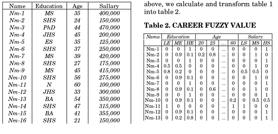
For example, given CAREER DATABASE in Table 1. By assuming that CAREER is a system which has 24 entries and three components, education, age, and salary, therefore Er=24, X=(X1:education, X2:age, X3: salary), Nm=CAREER. Now, we try to find relation among education, age, and
salary.
Table 1. CAREER DATABASE
Name Education Age Sallary
Nm-1 MS 35 400,000
Nm-2 SHS 24 150,000
Nm-3 PhD 44 470,000
Nm-4 JHS 45 200,000
Nm-5 ES 35 125,000
Nm-6 SHS 37 250,000
Nm-7 MS 39 420,000
Nm-8 SHS 27 175,000
Nm-9 MS 45 415,000
Nm-10 SHS 56 275,000
Nm-11 N 60 100,000
Nm-12 JHS 33 300,000
Nm-13 BA 54 350,000
Nm-14 SHS 47 315,000
Nm-15 BA 41 355,000
Nm-16 SHS 21 150,000
Nm-17 BA 52 374,000
Nm-18 PhD 49 500,000
Nm-19 ES 58 125,000
Nm-20 JHS 59 200,000
Nm-21 BA 35 360,000
Nm-22 SHS 37 255,000
Nm-23 BA 31 340,000
Nm-24 SHS 29 250,000
First, we classify all three domains or components as follows.
education = (low_edu,mid_edu,hi_edu),
age = (about_20,…,about_60), salary = (low_slr,mid_slr,hi_slr). where we assume that membership functions of low_edu, mid_edu, and
high_edu:
}. / 1 , / 1 , / 8 . 0 , / 1 . 0 { ) (
}, / 2 . 0 , / 9 . 0 , / 5 . 0 , / 2 . 0 { ) (
}, / 5 . 0 , / 8 . 0 , / 1 { ) (
PhD MS BA SHS
hi_edu
BA SHS
JHS ES
mid_edu
JHS ES
N low_edu
= = =
µ µ µ
Membership function of age,
)}. 4 /( 2 . 0
), 3 /( 4 . 0 ), 2 /( 6 . 0 ), 1 /( 8 . 0 , / 1 ), 1 /( 8 . 0
), 2 /( 6 . 0 ), 3 /( 4 . 0 ), 4 /( 2 . 0 { ) _ (
+
+ +
+ −
− −
− =
n
n n
n n n
n n
n n
about
µ
Membership function of low_salary, mid_salary, and high_ salary :
]. 300000 / 1 , 250000 /
0 [ ) (
], 0/300000
, 250000 /
1 , 150000 / 1 , 100000 / 0 [ ) (
], 150000 / 0 , 100000 / 1 , 0 / 1 [ ) (
= = =
hi_slr mid_slr low_slr
µ µ µ
By using all membership functions above, we calculate and transform table 1 into table 2.
Table 2. CAREER FUZZY VALUE
Education Age Salary
Nama
LE ME HE 20 25 … 60 LS MS HS
Nm-1 0 0 1 0 0 ... 0 0 0 1
Nm-2 0 0.9 0.1 0.2 0.8 ... 0 0 1 0
Nm-3 0 0 1 0 0 ... 0 0 0 1
Nm-4 0.5 0.5 0 0 0 ... 0 0 1 0
Nm-5 0.8 0.2 0 0 0 ... 0 0.5 0.5 0
Nm-6 0 0.9 0.1 0 0 ... 0 0 1 0
Nm-7 0 0 1 0 0 ... 0 0 0 1
Nm-8 0 0.9 0.1 0 0.6 ... 0 0 1 0
Nm-9 0 0 1 0 0 ... 0 0 0 1
Nm-10 0 0.9 0.1 0 0 ... 0.2 0 0.5 0.5
Nm-11 1 0 0 0 0 ... 1 1 0 0
Nm-12 0 0.9 0.1 0 0 ... 0 0 0 1
Nm-14 0 0.9 0.1 0 0 ... 0 0 0 1
Nm-15 0 0.2 0.8 0 0 ... 0 0 0 1
Nm-16 0 0.9 0.1 0.8 0.2 ... 0 0 1 0
Nm-17 0 0.2 0.8 0 0 ... 0 0 0 1
Nm-18 0 0 1 0 0 ... 0 0 0 1
Nm-19 0.8 0.2 0 0 0 ... 0.6 0 0.5 0.5
Nm-20 0 0.9 0.1 0 0 ... 0.8 0 1 0
Nm-21 0 0.2 0.8 0 0 ... 0 0 0 1
Nm-22 0 0.9 0.1 0 0 ... 0 0 0.9 0.1
Nm-23 0 0.2 0.8 0 0 ... 0 0 0 1
Nm-24 0 0.9 0.1 0 0.2 ... 0 0 1 0
Σ
3.1 10.9 10 1 1.8 ... 2.6 1.5 9.4 13.1Note: LE:low_edu, ME:mid_edu, HE = hi_edu, 20:about_20, 25:about_25, …, LS=low_slr, MS:mid_slr and HS:hi_slr. Definition 3.2 Xn is defined as compound attribute to express component of the system . Xn is a vector. If there are k elements of Xn then Xn=(xn1,…,xnk), where xni is element i of compound attribute Xn and for further, xni is called attribute. For example, if system CAREER has three compound attributes and their attributes as follows,
X1 : education = (low_edu,mid_edu,hi_edu),
X2 : age = (about_20,…,about_60),
X3 : salary = (low_slr,mid_slr,hi_slr).
then x11 =low_edu, x25 =about_40, etc.
Definition 3.3 ni j
e is defined as
member-ship’s value of entry j for attribute xni. If compound attribute Xn has k attributes then,
1 e j
k i 1
ni
j =
∀
∑
≤ ≤
(8)
Example, as shown in Table 2.,
,
9
.
0
,
5
.
0
122 11
4
=
e
=
e
etc.Definition 3.4 N(xni) is defined as sum of entries value for attribute xni. If there are Er number of entries, then
e
) x ( N
Er i 1
ni j
ni
∑
≤ ≤
= (9)
If compound attribute Xn has k attributes then,
) x ( N r E
k i 1
ni
∑
≤ ≤
= (10)
For example, as shown in Table 2.,
N(xni)=N(low_edu) = 3.1.
Definition 3.5 P(xni) is defined as probability of attribute xni as follows.
Er
)
x
(
N
)
x
(
P
nini
=
(11)If compound attribute Xn has k attributes then,
1 ) x ( P
k i 1
ni
∑
≤ ≤
= (12)
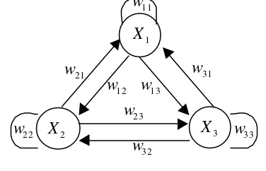
3.1 Relation Among Compound Attri-butes
Given three compound attributes, X1, X2 and X3. Relation among them can be illustrated in Fig. 1. as follows.
Figure 1. Relation Among Compound Attributes, X1, X2 and X3.
Definition 3.6 wnm is defined as weight matrix, to express degree of dependency of
Xm from Xn. For a k-compound attribute Xn and a j-compound attribute Xm, wnm and wmn present two different matrices, as follows.
.
,
2 1
2 22
21
1 12
11 2 1
2 22
21
1 12
11
=
=
mn jk mn
j mn j
mn k mn
mn
mn k mn
mn
mn
nm kj nm
k nm k
nm j nm
nm
nm j nm
nm
nm
a
a
a
a
a
a
a
a
a
w
a
a
a
a
a
a
a
a
a
w
L M O M M
L L L
M O M M
L L
Definition 3.7 Each element of matrix
wnm, entry aihnm expresses numerical probabilistic value of relation from xni∈Xn
1
X
2
X
X
321
w
12
w
22
w
31
w
13
w
33
w
11
w
23
w
32
to xmh∈Xn. nm ih
a can also be interpreted as conditional probability as follows.
)
If there are Er number of entries, then
e
a expresses
numerical probabilistic value of relation from xmh∈Xm to xni∈Xn. mn
hi
a can also be interpreted as conditional probability as follows.
If there are Er number of entries, then
e
From equations (13), (14) and (15), (16), we conclude that mn
hi
a and nm ih
a are in general different.
The above definition leads to the conclusion that every attribute can be used to determine itself perfectly.
3.2 Relation Among Attributes In System
Given three attributes, x1u∈X1,
2
2 X
xv∈ and x3r∈X3. Relation among
these three attributes can be seen in Fig. 2.
Figure 2. Relation Among Attributes, x1u,
x2v, and x3r.
In order to understand the meaning of this connection, we use relation of set.
the same area or quantity, are inter-section between x1u and x3r. In the same way, we can find two other relations,
)
which are proved as follows.
From the relations above, we find the following equation.
a
a
.
a
a
a
.
a
31 ru
13 ur 21 vu 32
rv 23 vr 12
uv
=
(19)
Proof:
.
) (
) (
,
31 13 21 32 23 12
31 3 13 21 32
3 23 12
1 21 2 12
ru ur vu rv vr uv
ru r ur vu rv
r vr uv
u vu v uv
a a a a a a
a ) P(x a a a
) P(x a a
) P(x a ) P(x a
⋅ = ⋅
⋅ ⋅ = ⋅
⋅
⋅ = ⋅
Important characteristic of relation among attributes is transitive relation, i.e. given 12
uv
a
, 21vu
a
, 23vr
a
, 32rv
a
and we would like to find interval value ofa
13ur, which satisfy the two following equations.Lower bound of 13
ur
a
,.
a
a
)}.
1
a
a
(
,
0
max{
a
32rv 23 vr 32
rv 12 uv 13
ur
≥
+
−
(20)Upper bound of 13
ur
a
,. a a }. a a ). a 1 ( , a a ). a -min{(1
a
a }. a , a min{ a
32 rv 23 vr 23 vr 32 rv 23 vr 21
vu 12 uv 21 vu
32 rv 23 vr 12 uv 32 rv 13
ur
− + ≤
(21)
Proof :
To find the upper bound of
a
13ur, first we take the maximum area insidex
2v, resultof intersection between two intersection areas which are intersection between
x
1u andx
2v, expressed in 12uv
a
and intersection betweenx
3randx
2v, expressed in 32rv
a
. The maximum area that is result of overlapping between the two intersection areas, shown in Fig. 3., can be expressed in min function applied toa
12uvanda
32rv. The next, we plus with maximum intersection between remainx
1uandx
2v which be outside ofx
2v. Again, this area can be expressed in min function applied to(
1
−
a
vu21)
and(
1
−
a
vr23)
. Value of these two area point to two different area,x
1uand
x
3r. However, in order to be able to becompared, they must be point to the same area, in this case we use
x
2v as base for their comparison. Therefore, we must convert them intox
2v by multiplying with21 12
vu uv
a
a
and 23
32
vr rv
a
a
, respectively. Finally, again we must convert all from
x
2v intox
3rby multiplying with 2332
vr rv
a
a
.
Figure 3. Maximum Area of Intersection between
x
1u andx
3r insidex
2v.To find the lower bound of 13
ur
a
, we take the minimum area insidex
2v, result of intersection between two intersection areas which are intersection betweenx
1u andx
2v, expressed in 12uv
a
and intersection betweenx
3r andx
2v, expressed in 32rv
a
. The minimum area which is result of as much as possible avoid overlapping between the two intersection areas, shown in Fig. 4., can be expressed in max function applied to 12uv
a
and 32rv
a
as shown in (13). The next, we convert quantity of the maximum area fromx
2v intox
3r by multiplying with 2332
vr rv
a
a
.
Figure 4. Minimum Area of Intersection between
x
1u andx
3r insidex
2v.12 12 32
) ,
min(arv au v =au v
23 32 23
23 32 23
21 12 21
) 1 (
} ) 1 (
, ) 1 min{(
vr rv vr
vr rv vr
vu uv vu
a a a
a a a
a a a
⋅ − =
⋅ −
⋅ −
v
x
2r
x
3u
x
1) 1 (
)) 1 (
, 0 max(
12 32
12 32
− + =
− +
uv rv
uv rv
a a
a a
v
x
2r
x
3u
4. CALCULATING PREDICTION After constructed the model of system, it can be used to predict interval probability (find lower and upper bound) of any query data. In this section, we generate formulas to calculate interval probability of the query data. First, user must give input related to data type of compound attributes.
Definition 4.1 Q is define as set of input data that be given by user to do query for a certain data. If there are n
compound attributes then Q={q1,…,qn} where qi is data input related to compound attribute Xi.
For example, suppose CAREER system has been constructed, given John is old man and has MS degree as input for
age and education, respectively, then q1 = old and q2=MS.
Definition 4.2 P(Xi,qi) is defined as probabilistic matching of compound attribute Xi toward given input data qi. If there are k elements or attributes of compound attribute Xi, then,
P(Xi,qi)=( pi1,…, pik), (22) where
pij= P(xij|qi), (23) expresses conditional probability for xij given qi. In this case Point Semantic Unification Process [1,3] can be used to calculate pij.
For example, given qi =old which is a fuzzy set defined as qi ={0/55,1/60}.
Xi = age has 9 attributes as defined in section 2, as follows.
Xi = {about_20,about_25,…,about_60}. By using point semantic unification process applying to membership function of age which has been defined in section 2 and membership function of qi, we calculate P(Xi,qi) as follows. First, we calculate the mass assignment for qi. It is equivalent to the basic probability assignment of Dempster Shafer Theory which we can write as
0.2. : {60} 0.2, : {59,60} 0.2,
: {58,59,60}
, 2 . 0 : } 60 ,... 57 { , 2 . 0 : } 60 ,..., 57 , 56 {
= i q
m
Next, i.e. mass assignment for xi8=55 as one attribute of Xi is given by
0.2. : {55} 0.2, : {54,55,56} 0.2,
: } {53,...,57
, 2 . 0 : } 58 ,... 52 { , 2 . 0 : } 59 ,..., 51 {
8 =
i
x
m
Process to calculate Point Value Semantic Unification of relation between two fuzzy set, old and about_55 or P(about_55,old) is shown in the following table.
0.2 0.2 0.2 0.2 0.2
{56,…,60} {57,…,60} {58,59,60} {59,60} {60} 0.2
{51,...,59} 0.032 0.03 0.026 0.02 0
0.2
{52,...,58} 0.024 0.02 0.013 0 0
0.2
{53,...,57} 0.016 0.01 0 0 0
0.2
{54,55,56} 0.008 0 0 0 0
0.2
{55} 0 0 0 0 0
From the table, we calculate
0.199.
0.008 0.01
0.016 0.013 0.02 0.024
0.02 0.026 0.03 .032 0 ) , 55 _ (
= +
+ + + +
+ + + + =
old about P
In the same way, we find P(about_ 60,old) = 0.799, where P(about_20,old) = P(about_25,old) = ... = P(about_50,old) = 0, because there is no intersection between their members. Finally, we find,
). 799 . 0 , 199 . 0 , 0 , 0 , 0 , 0 , 0 , 0 , 0 ( ) , ( )
(X,q =P ageold =
P i i
Definition 4.3
P
(
X
i,q
j)
is defined as probability of attributeX
i,influenced by given input dataq
j.X
i andq
j have different type of data, therefore to find their probabilistic matching, first, we must findP
(
X
j,q
j)
and then apply max-multiply (*) operation betweenP
(
X
j,q
j)
(27) defined as probability of attribute
x
ir influenced by given set input data Q, is∨
operation for all probabilities of relation betweenx
ir and all members of Q.∨
operation will be explained in the latter. If there are n members of Q,{(
q
1,...,
q
n)}
, probability of compound attributeX
i influenced by given set input data Q. If there are n members of Q and k4.1 Calculating minimum probability truth of
P
(
x
ir,Q
)
Now, we generate formula for calcu-lating minimum probability of attribute
ir
x
givenQ
=
{
q
1,...,
q
n}
, as input data. Related to (27), we defined minimum probability truth ofP
(
x
ir,
Q
)
as follows.To simplify the problem, let’s say that system just has three compound attri-butes,
X
1,
X
2,
andX
3 and their relationshown in Fig. 2. We calculate minimum probability truth of
x
3r∈
X
3 based onWe separate formula above into two parts. The first, we call direct predicted probability of
x
3r which iswe call indirect predicted probability truth of
x
3r which is predicted from other attributes value,P
(
x
3r,q
1)
∨
minP
(
x
3r,q
2)
. The next, we compare both of them by applying max function as follows.)}.
The problem now, is how to calculate
.
attributes,
X
2 has t attributes. Let’s say that,2. If
|
(
x
3r∩
x
2v)
|
≤
|
(
x
1u∩
x
3r)
|
andFrom the above conditions, we gene-rate a formula that satisfy all conditions as follows.
(33)
Finally, we find that
)}.
4.2 Calculating Maximum Probability Truth of
P
(
x
ir,
Q
)
Next, we generate formula for calcu-lating maximum probability of attribute
xir given Q=(q1,… qn), as input data.
Related to (27), we defined maximum probability truth of
P
(
x
ir,
Q
)
as follows.To simplify the problem, let’s say that system just has three compound attributes, X1, X2 and X3 and their relation shown in Fig. 2.2. We calculate maximum probability truth of
x
3r∈
X
3We separate formula above into two parts. The first, we call direct predicted probability of x3r which is P(x3r|q3) = P(x3r|q3) = p3r and the second, we call indirect predicted probability truth of x3r which is predicted from other attributes value, P(x3r,q1)∨maxP(x3r,q2) . The next, we
compare both of them by applying min
function as follows.
)}
The problem now, is how to calculate
max
)
From the above conditions, we generate a formula that satisfy all condition as follows.
Finally, we find that
)}.
5. CONCLUSION
This paper proposed a method based on conditional probability relation to approximately calculate interval proba-bility of dependency of data for data querying. Theoretically the formulation is quite interesting. However, it seems to be too complicated to calculate interaction of three or more components. Practically the formulas should be simplified, even though the accuracy of prediction may be decreased.
REFERENCES
1. Intan, R., Mukaidono, M., ‘Application of Conditional Probability in Con-struc ting Fuzzy Functional Depen-dency (FFD)’, Proceedings of AFSS’00, 2000, pp.271-276.
2. Intan, R., Mukaidono, M., ‘A proposal of Fuzzy Functional Dependency based on Conditional Probability’,
3. Intan, R., Mukaidono, M., ‘Fuzzy Functional Dependency and Its Application to Approximate Query-ing’, Proceedings of IDEAS’00, 2000, pp.47-54.
4. Intan, R., Mukaidono, M., ‘Condi-tional Probability Relations in Fuzzy Relational Database ’, Proceedings of RSCTC’00, LNAI 2005, Springer & Verlag, 2000, pp.251-260.
5. Baldwin J.F., ‘Knowledge from Data using Fril and Fuzzy Methods’,Fuzzy Logic,John Wiley & Sons Ltd 1996, pp. 33–75.
6. Yukari Yamauchi, Masao Mukaidono , ‘Interval and Paired Probabilities for Treating Uncertain Events’, The Institute of Electronics, Information and Communication Engineers, Vol. E82-D (May 1999), pp. 955–961. 7. Baldwin J.F., Martin T.P., and
Pilsworth B.W. FRIL-Fuzzy and Evidential Reasoning in AI, Research Studies Press and Willey, 1995.
8. Shafer G. A Mathematical Theory of Evidence, Princeton Univ. Press. 1976.
9. Richard Jeffrey, ’Probabilistic Think-ing’, Priceton University, 1995.