www.elsevier.nl/locate/cam
QD-algorithms and recurrence relations for biorthogonal
polynomials
(Zelia da Rocha∗;1
Departamento de Matematica Aplicada, Faculdade de Ciˆencias, Universidade do Porto, Rua das Taipas 135, 4050 Porto, Portugal
Received 9 December 1998
Abstract
Biorthogonal polynomialsPn(i; j)include as particular cases vector orthogonal polynomials of dimensiondand−d(d∈N).
We pay special attention to the cases of dimension 1 and−1. We discuss the problem of computingPn(i; j)using only one
or several recurrence relations. Furthermore, we deduce all recurrence relations of a certain type that givePn(i; j) from two
other biorthogonal polynomials. The coecients that appear in any two independent relations satisfy some identities from which it is possible to establish QD-like algorithms. c1999 Elsevier Science B.V. All rights reserved.
MSC:41A21; 42C05
Keywords:Biorthogonal polynomial; Vector orthogonal polynomial of dimensiondand −d(d∈N); Recurrence relation; QD-algorithm
1. Introduction
In this paper, we begin by recalling the notion of biorthogonal polynomials P(i; j)
n [2]. These
polynomials are dened from a general sequence of linear functionals {Li}i=0;1;:::, that only have to
be linearly independent. Biorthogonal polynomials are in the base of a generalisation of Pade-type approximants for a series of functions [2]. Vector orthogonal polynomials of dimension d and
−d (d∈N) are particular cases of biorthogonal polynomials obtained making suitable hypothesis on the functionals Li. In fact, all the sequence {Li}i=0;1;::: is determined from d functionals.
Vector orthogonal polynomials of dimension d [11] appear in the construction of vector Pade approximants that are rational approximants of d functions given by their Maclaurin series [10,12].
(
Financial support from Fundac˜ao Ciˆencia e Tecnologia, Portugal.
∗Tel: ++351-2-2080313; fax: ++315-2-2004109.
E-mail address: [email protected] (Z. da Rocha)
1Also Centro de Matematica Aplicada da Universidade do Porto; Rua das Taipas, 135; 4050 Porto; Portugal.
Vector orthogonal polynomials of dimension −d [5] arise naturally in the determination of rational approximants of d Laurent series [14].
The computation of biorthogonal polynomials can be made using only one recurrence relation. We discuss the implementation of that relation, and we give the detail of the elements that have to be calculated and stored in the memory. The total amount of these elements grow quickly, so some problems of space of memory and time of execution can arise.
Another possibility is to use simultaneously several recurrence relations in order to store in the memory a xed number of polynomials. This technique was employed with success in the devel-opment of a program for the computation of the table of Pade approximants [1].
Using an exhaustive method, we deduce all recurrence relations of a certain type between three biorthogonal polynomials. But, we realise that, in the general case, it is not possible to chain the relations. Otherwise, if we consider these relations in the cases of vector orthogonal polynomials of dimension 1 and −1, we can apply alternatively several relations in order to compute some sequences or even the table of the corresponding polynomials, storing in the memory a xed number of polynomials.
Four of the 12 relations that we get for biorthogonal polynomials have already been found in [2], using the Sylvester and Schweins’s identities of determinants. In fact, only two of these relations are independent, and it is possible to deduce the others from these two.
The coecients that appear in any two independent relations are connected by two identities from which we can establish algorithms to get the corresponding coecients. We call them QD-like algorithms, because some of them look like the QD-algorithm for orthogonal polynomials [16]. It is possible to establish several versions of the algorithms and write them in direct and progressive forms.
The implementation of QD-algorithms presents the same problems as the computation of biortho-gonal polynomials from one recurrence relation. There is a signicant amount of elements to compute and store that grows quickly.
2. Biorthogonal polynomials
Let {Li}i=0;1;::: be a sequence of linear functionals on the space of complex polynomials, and let {xi}
Let us suppose that we are in the normal case, that is,
D(i; j)
This condition is equivalent to the condition
{Li}i=0;1;::: is an independent linear family;
since {xi}
i=0;1;::: is an independent linear family [8].
Let us dene the so-called adjacent biorthogonal polynomials from the equality
Pn(i; j)(x) =Nn(+1i; j)(x)=D(ni; j): (1)
It is easy to see that P(i; j)
n is a monic polynomial of degree n that satises the n following
biorthogonality conditions:
Lp(xjPn(i; j)(x)) = 0; p=i; : : : ; i+n−1: (2)
In the normal case, every monic polynomial of degree n that satises these conditions is equal to P(i; j)
n .
This denition was given by Brezinski [2]. From (1), we obtain the following equalities:
Li−1(x
jP(i; j)
n ) = (−1)
nD(i−1; j)
n+1 =D (i; j)
n ;
Li+n(xjPn(i; j)) =D
(i; j)
n+1=D(ni; j);
P(i; j)
n (0) = (−1)
nD(i; j+1)
n =D
(i; j)
n :
Then, in the normal case
Li−1(x
jP(i; j)
n )6= 0; Li+n(xjPn(i; j))6= 0 and Pn(i; j)(0)6= 0; (3)
which means that the biorthogonality conditions of P(i; j)
n can not be extended to p=i−1 nor
p=i+n, and that the independent term of these polynomials does not vanish.
3. Particular cases
3.1. Vector orthogonal polynomials of dimension d (d∈N)
Let L0; : : : ; Ld−1 be d linear functionals on the space of complex polynomials, and let us dene the functionals of a greater order as follows:
Lp(xk) =Ldq+r(xk) =Lr(xk+q);
where p¿d and q and r are the quotient and the remainder of the division of p by d. Let us write the determinants Nn(+1i; j)(x) and D(i; j)
n in this particular case.
We begin by calculating the quotient qi and the remainder ri of the division of i by d, and the
quotient q and the remainder r of the division of n−d+ri by d:i=dqi+ri; where 06ri¡ d and
We obtain
n as the determinant constituted by the n rst rows and columns of N
(i; j)
n+1(x).
We see that the biorthogonality conditions of P(i; j)
n can be written as follows:
Lp(xj+qiPn(i; j)(x)) = 0; p=ri; : : : ; d−1;
(d; n) are the generalized Hankel
deter-minants in the sense of Van Iseghem [11] and {P(j+qi)
(d; n) }n¿0 is the family of the monic
(j+qi)-adjacent vector orthogonal polynomials of dimension d(d∈N), with respect to {Lr}r=0;:::;d−1. These polynomials were dened and studied by Van Iseghem [11], who showed that they satisfy a Shohat–Favard theorem and that the family {P((d; nk))}n¿0 satises a recurrence relation of orderd+1,
and that the two families {P((d; nk))}n¿0 and {P((d; nk+1)) }n¿0 are related by a vector QD-algorithm. Other
relations involving d+ 2 polynomials can also be found (see [13]). These polynomials are used in the construction of vector Pade approximants, that are rational approximants to d functions given by their Maclaurin developments (see [10,12]).
3.1.1. Vector orthogonal polynomials of dimension 1
In the case d= 1, we start from only one linear functional L≡L0. Functionals of greater order
are dened as follows:
Lp(xk) =L(xk+p); p; k∈N0:
Lp is usually denoted by L(p).
Nn(+1i; j)(x) =
n is the determinant constituted by the n rst rows and columns of N
(i; j)
n+1(x), as usual.
We realize that D(i; j)
n is the Hankel determinant Hn(i+j), and that the biorthogonality conditions of
P(i; j)
orthogonal polynomials with respect to L, that is the family of the monic orthogonal polynomials with respect to L(i+j) (see [1]).
If i=j= 0, P(0;0)
n ≡Pn(0)≡Pn; where {Pn}n¿0 is the family of monic orthogonal polynomials with
respect to L:
3.2. Vector orthogonal polynomials of dimension −d(d∈N)
Let L0; : : : ; Ld−1 be d linear functionals on the span{xl; l∈Z}, and let us dene the linear func-tionals Lp on the space of complex polynomials as follows:
Lp(xk) =Ldq+r(xk) =Lr(xk−q); p; k∈N0;
where q and r are the quotient and the remainder of the division of p by d. We remark that in this case, we use upper indexes in the rst d functionals. Let us write the determinants Nn(+1i; j)(x) and D(i; j)
n as the determinant constituted by the n rst rows and columns of N
(i; j)
We see that the biorthogonality conditions of P(i; j)
n can be written as follows:
Lp(xj−qiP(i; j) (j − qi)-adjacent vector orthogonal polynomials of dimension −d (d∈N), with respect to {Lr}
r=0;:::;d−1.
These polynomials were dened and studied by Brezinski and Van Iseghem [5], who showed that they satisfy a Shohat–Favard theorem, that the family {P([k]
−d; n)}n¿0 satises a recurrence relation of orderd+1, and that two families{P([k]
−d; n)}n¿0 and{P
[k−1]
(−d; n)}n¿0 are related by a vector QD-algorithm. These polynomials are used in the construction of rational approximants to d functions given by their Laurent developments (see [14]).
3.2.1. Vector orthogonal polynomials of dimension −1
In this case, we have only one linear functional L≡L0 dened on span{xl; l∈Z}. The linear
functionals Lp on the space of complex polynomials are dened as follows:
Lp(xk) =L(xk−p); p; k∈N0:
n is the determinant constituted by the n rst rows and columns of N
(i; j)
n+1(x).
We see that the biorthogonality conditions of P(i; j)
n can be written as follows:
L(xj−i−pP(i; j)
n ) = 0; p= 0; : : : ; n−1:
These polynomials only depend on the dierence j−i and thus P(i; j)
n ≡Pn[j−i], where {Pn[j−i]}n¿0
is the family of monic (j−i)-adjacent vector orthogonal polynomials of dimension −1 with respect to L. We denote D(i; j)
n by Hn[j−i], and we remark that j−i∈Z.
These polynomials were dened and studied by Brezinski [3], who showed that they satisfy a Shohat–Favard theorem, a Christoel–Darboux-type formula and several recurrence relations. Brezin-ski and Redivo Zaglia [4] have written the recurrence relation of order two in the nonnormal case.
4. Computing biorthogonal polynomials from one recurrence relation
Let us treat the problem of computing biorthogonal polynomials. Of course, we should not use directly expression (1), that gives P(i; j)
n as a ratio of determinants.
deduce recurrence relations that, with suitable initial conditions, allow to compute recursively some polynomials from the others.
Given the linear functionals {Li}i=0;1;:::, the computation of the sequence {P(ni; j)}n=0;1;:::, with the
indexes i and j xed, can be done from the initial conditions
P0(i; j)(x) = 1; ∀i; j∈N0; (4)
using only the following relation:
P(i; j)
n (x) =xP
(i; j+1)
n−1 (x) +
Li+n−1(x
j+1P(i; j+1)
n−1 ) Li+n−1(x
jP(i; j) n−1)
Pn(i; j)
−1(x): (5)
This relation was deduced by Brezinski [2], from expression (1), using the Sylvester’s identity for determinants.
The problem is that, using only one relation, a lot of elements that do not interest us have to be computed. More precisely, the computation of the n+ 1 polynomials {Pk(i; j); k= 0; : : : ; n} requests the computation of the following elements that we dispose in the n+ 1 arrays corresponding to the dierent values of k.
These arrays have a total amount of Pn+1
i=1 i2 ≈ O(n3=3) elements. We remark that this number
depends on n.
The initial conditions (4) and relation (5) can be easily implemented in theMathematicalanguage [9,15], in a recursive way as follows:
bp[i ; j ;0; var ] :=bp[i; j;0; var] = 1;
var∗bp[i; j+ 1; n−1; var]−
lf[i+n−1; var∧(j+ 1)∗bp[i; j+ 1; n−1; var]; var]=
lf[i+n−1; var∧j∗bp[i; j; n−1; var]; var]∗
bp[i; j; n−1; var];
where we take, for example
lf[i ;body ; var ] :=lf[i;body; var] =Function[var;body][−1=(i+ 1)]
as the denition of the linear functional Li(f) =f(−1=(i+ 1)).
Given the above Mathematicadenitions, in order to compute {Pk(1;2); k=0; : : : ;20}, for example, we simply write
Do[ bp[1;2; k; x];{k;0;20}]:
This kind of Mathematica denitions [15, p. 225] uses the following principle: every element that is called, is calculated by the recurrence denition, and is stored permanently in the memory, in case it is needed later. In this example, all the elements corresponding to the arrays P0; : : : ; Pn are
calculated and stored in the memory permanently. In this manner, Mathematica never repeats the same computation, but lls in the memory with elements, such that eventually it does not need any more to continue the computations. Furthermore, if the number of elements to store grows too fast, an error, “out of memory”, can be quickly produced.
So, we should use a kind of implementation that, in each step, makes out the dierence between the elements that will be needed in the sequel of computations, and the elements that can disappear. This principle was employed by da Rocha [6,7] to make an iterative implementation of some recurrence relations of biorthogonality that are similar to the one we treat here. Using this principle the number of elements to store is about O(n2).
5. Computing biorthogonal polynomials from several recurrence relations
In this section, our idea is to use simultaneously several recurrence relations in order to calculate some sequences of biorthogonal polynomials storing in the memory a xed number of polynomials. The rst step to do that is to deduce other relations.
Let us represent P(i; j)
n in the space by the point of co-ordinates (i; j; n).
We say that the two polynomials P(i1; j1)
n1 and P (i2; j2)
n2 , i1; j1; n1; i2; j2; n2∈N0 are consecutive
adja-cent biorthogonal polynomials or neighbouring biorthogonal polynomials if and only if |i1−i2|61,
|j1−j2|61 and |n1−n2|61:
Let us nd all recurrence relations that allow the calculation of P(i; j)
n from two of its consecutive
adjacent polynomials. That is, we look for all the relations of the following type:
Pn(i; j)(x) =f1(x)Pn(1i1; j1)(x) +f2(x)P (i2; j2)
n2 (x); (6)
where the indexes i1 and i2 can only take the values i−1, i or i+ 1; the indexes j1 andj2 can only
and the factors f1 and f2 are as follows:
f1(x) =
k2
X
m1=−k1
am1x
m1; f 2(x) =
k4
X
m2=−k3
bm2x m2; k
1; k2; k3; k4∈N0:
It is obvious that the three polynomials that appear in relation (6) must be dierent.
In the normal case, this relation exists if and only if the right-hand side of (6) represents a monic polynomial of degree n, that satisfy the biorthogonality conditions (2).
Let us see how to determine the coecients am1 and bm2, and the indexesi1; i2; j1; j2; n1 andn2.
We begin by writing down the biorthogonality conditions
k2
X
m1=−k1
am1Lp(x
j+m1P(i1; j1) n1 ) +
k4
X
m2=−k3
bm2Lp(x
j+m2P(i2; j2)
n2 ) = 0; p=i; : : : ; i+n−1: (7)
Fixing the indexes i1, i2, j1, j2, n1 and n2, these conditions form a system of n homogeneous,
linear equations with respect to k1+k2+k3+k4+ 2 unknowns {am1} k2
m1=−k1 and {bm2} k4 m2=−k3.
If j1=j+m1 andj2=j+m2, the biorthogonal conditions ofPn(1i1; j1) andP (i2; j2)
n2 can be employed, and
the number of equations of system (7) become xed, that is, does not depend on n. If j16=j+m1
or j2 6=j+m2, then in the general case, the biorthogonality conditions of Pn(1i1; j1) or P (i2; j2)
n2 can not
be employed, and system (7) will have a number of equations that is not xed. To suppose that this system is consistent is equivalent to supposing additional conditions on the functionals Lis. We
exclude this eventuality, because we want to work in the general case.
So, we require that j1=j+m1 and j2=j+m2. This implies that, xing j1 and j2, ∃!m1:am1 6= 0
and ∃!m2 :bm2 6= 0. Furthermore, as j1 and j2 can only take the values j−1, j and j+ 1, the values
of m1 and m2; such that am1 and bm2 do not vanish, much be chosen among −1; 0 and 1. So,
f1(x) =axm1 and f2(x) =bxm2;
where a and b do not vanish, and m1 and m2 are equal to −1, 0 or 1.
Then, relation (6) and the biorthogonality conditions (7) become as follows:
Pn(i; j)(x) =axm1P(i1; j+m1)
n1 (x) +bx
m2P(i2; j+m2)
n2 (x); (8)
aLp(xj+m1Pn(1i1; j+m1)) +bLp(x
j+m2P(i2; j+m2)
n2 ) = 0; p=i; : : : ; i+n−1: (9)
It remains to determine a; b; i1; i2; m1; m2; n1 and n2:
Let us begin by xing the degrees n1 and n2: There are several cases to consider:
1. The two degrees are equal to n−1: n1=n2=n−1:
2. The two degrees are equal to n:n1=n2=n:
3. The two degrees are equal to n+ 1: n1=n2=n+ 1:
4. One of the degrees is equal to n and the other is equal to n−1: for example n1=n; n2=n−1:
5. One of the degrees is equal to n and the other is equal to n+ 1: for example n1=n; n2=n+ 1:
6. One of the degrees is equal to n+ 1 and the other is equal to n −1: for example n1 =
n+ 1; n2=n−1:
In each case, the values of n1 and n2 enable us to determine the possible values of m1 and m2, in
of possible values of m1 and m2, the fact that Pn(i; j), Pn(1i1; j+m1) and P (i2; j+m2)
n2 are monic enable us to
x one of the coecients a or b, or even both.
It remains to determine the indexes i1 and i2 and perhaps one of the coecients a or b, if they
have not already been determined.
Let us consider now all the possible values of the indexes i1 and i2:
The biorthogonality conditions of P(i1; j+m1) n1 and P
(i2; j+m2) n2
Lp(xj+m1Pn(1i1; j+m1)) = 0; p=i1; : : : ; i1+n1−1;
Lp(xj+m2Pn(2i2; j+m2)) = 0; p=i2; : : : ; i2+n2−1;
imply that the biorthogonality conditions (9) are veried for p=p1; : : : ; p2, where
p1= max{i1; i2} and p2= min{i1+n1−1; i2+n2−1}:
From all the possible values of i1, i2, n1 and n2, we know that p1¿i−1 and p26i+n+ 1:
Let us see that the cases p1=i−1, p2=i+n and p2=i+n+ 1 are not possible.
If p1=i−1 or p2=i+n, then we get
Li−1(x
jP(i; j)
n ) = 0 or Li+n(xjPn(i; j)) = 0;
which is impossible, since we are in the normal case (see (3)).
If p2=i+n+ 1;which is equivalent to i1=i2=i+ 1 and n1=n2=n+ 1; then m1 andm2 must be
dierent, otherwise P(i1; j+m1) n1 ≡P
(i2; j+m2)
n2 , which is impossible. Then, we have three possibilities for
the values of the indexes m1 andm2, namely one of the index is equal to −1 and the other is equal
to 0, for example m1=−1 and m2= 0; one of the index is equal to −1 and the other is equal to 1,
for example, m1=−1 and m2= 1; and nally one of the index is equal to 0 and the other one is
equal to 1, for example m1= 0 and m2= 1: It is easy to see that in all these cases, the right-hand
side of (8) represents a polynomial of degree greater than n, which is impossible. Then, p1¿i and p26i+n−1:
Ifp1=iandp2=i+n−1, then the biorthogonality conditions (9) are veried, and the corresponding
relation (8) exists.
If p1 6=i or p26=i+n−1, the biorthogonality conditions corresponding to
p=i; : : : ; p1−1 or p=p2+ 1; : : : ; i+n−1
are not ensured.
If one of the coecients a or b remains to be determined, it must satisfy the system formed by the biorthogonality conditions corresponding to these values of p. If this system is impossible, relation (8) does not exist.
With this exhaustive procedure, we nd 12 relations that we number in the order of their appear-ance as, F1; : : : ; F12.
There are no other relations of this type.
The coecients that appear in Fk are denoted by C
(i; j; n)
(k; l) ; l= 1;2, where i,j andn are the indexes
F8: Pn(i; j)(x) =C
Relations F1, F2, F5 and F6 have already been found by Brezinski [2] using the Sylvester and
Schweins’s identities of determinants.
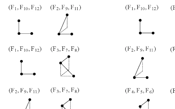
We remark that these relations are not independent. In fact, it is easy to prove that
F1 ⇔F10⇔F12; F2 ⇔F9⇔F11; F6⇔F5 ⇔F4 and F8⇔F7 ⇔F3:
Thus, we divide the relationsF1; : : : ; F12in four groups, namely{F1; F10; F12},{F2; F9; F11},{F6; F5; F4}
and{F8; F7; F3}, and we choose F1, F2, F6 and F8 as representatives of each set of relations. This
is an arbitrary choice.
Furthermore, the four groups of relations are not independent. In fact, we can prove that
Fig. 1. Trying to chain two independent relations.
F1 and F8 ⇒F2 and F6; F2 and F6⇒F1 and F8;
F2 and F8 ⇒F1 and F6; F6 and F8⇒F1 and F2:
In conclusion, there are only two independent relations.
We are going to show that it is not possible to compute any sequence of biorthogonal polynomials using alternatively several recurrence relations.
Let us denote by Fi andFj any two independent relations. In Fig. 1, we represent the combinations
of any two independent relations. As it is easy to see, we can never applyFi,Fj and afterFi, in order
to obtain new polynomials. In other words, it is not possible to chain two independent relations. Starting from the initial conditions P0(i; j)≡1; ∀i; j∈N; we realize that F1 and F2 are the only
relations that allow to get a polynomial of degree greater than 0, that is, they are the only relations that allow to leave the initial plane n= 0.
We represent by p and q the polynomials in the left-hand side of F1 and F2, and we represent
by r and s the polynomials in the right-hand side of those relations, respectively. Applying the 12 relations F1; : : : ; F12 to the polynomials p; q; r and s, we get
F3: (s; r)→p; F6: (q; r)→s; F9: (s; q)→p; F12: (r; p)→q;
F4: (s; r)→q; F7: (p; s)→r; F10: (r; q)→p; F1: (p; q)→r;
F5: (q; s)→r; F8: (p; r)→s; F11: (s; p)→q; F2: (p; q)→s:
We realise that we are in a cycle formed by the polynomials p; q; r and s, and that it is not possible to get other polynomials.
Nevertheless, in the particular cases of vector orthogonal polynomials of dimension 1 and −1, this idea can be applied with success.
6. Recurrence relations for vector orthogonal polynomials of dimension d and −d (d∈N)
We can easily write the formulas obtained in the preceding section in these particular cases. In each relation, we must convert the polynomials and write the new expressions of the coecients.
If d ¿1, the formulas that relate only vector orthogonal polynomials are F1; F10 and F12, because
all the left upper indexes of the polynomials that appear in these formulas are equal. Remember that in Sections 3.1 and 3.2, we write i=dqi+ri, and ri must vanish in order to get Pn(i; j)≡P
In both cases, F1 is one of the relations that determine the vector QD-algorithm (in the case of
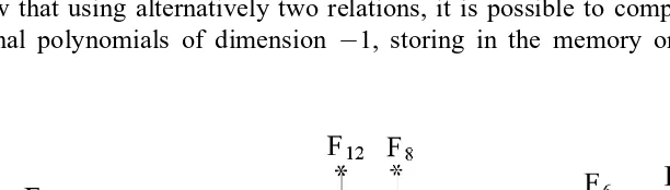
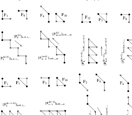
dimension d see [11], in the case of dimension −d see [5]). When d= 1, the twelve relations F1; : : : ; F12 exist. appears in the left-hand side of the formulas, and the dots • indicate the polynomials that are in the right-hand side. The polynomials P(m)
n are placed as usual, that is the lower index n is constant
on a vertical line, and the upper index m is constant on a descending diagonal. Some of these relations corresponding to the polynomials ˜Pn(m)(x) = xnP(m)
n (1=x), in the normal case, have been
used by Brezinski [1], to compute the table of Pade approximants storing in memory only three approximants at each time.
n . We remark that, we do not get exactly the same relations as in the case of orthogonal
polynomials. On the other hand, from these relations, it is possible to deduce other ones easily. In Fig. 4, we show that using alternatively two relations, it is possible to compute several sequences of vector orthogonal polynomials of dimension −1, storing in the memory only three polynomials at
Fig. 3. Relations between three consecutive vector orthogonal polynomials of dimension−1.
each time. We can also use the set of relations to compute the table of P[m]
n , storing a xed number
of polynomials in the memory. A similar situation occurs in the case of dimension 1.
7. QD-algorithms
In this section, we deal with the coecients Ck(i; j; n) that appear in F1; : : : ; F12.
As we have done with the relations, we divide the coecients into four groups, namely {C1; C10;
C12};{C2; C9; C11}; {C6; C5; C4} and {C8; C7; C3}:
When we prove, for example, that F1 ⇔F10 ⇔F12, we obtain
C10(i; j; n)=−C(i; j−1; n+1)
1 ; C
(i; j; n)
1 =−1=C (i; j; n−1)
12 ; C
(i; j; n) 1 =−C
(i; j+1; n−1)
10 ;
C12(i; j; n)=−1=C1(i; j; n+1); C10(i; j; n)= 1=C(i; j−1; n)
12 ; C
(i; j; n) 12 = 1=C
(i; j+1; n) 10 :
These identities mean that it is possible to write each of the coecients C1; C10 andC12 in terms
of each of the other two.
A similar situation occurs, since we proved the equivalences between the other recurrence rela-tions.
In conclusion, we can say that in each set of coecients, every coecient can be written in terms of each of the other two.
As we have done with the relations, let us chose C1; C2; C6 and C8 to represent the groups of
coecients.
With respect to the implications between the relations, when we prove, for example, that F1 and
F2 ⇒F6 and F8, we obtain
C6(i; j; n)=C2(i; j; n)−C1(i+1; j; n); (10)
C(8(i; j; n;1))=C2(i; j; n)=C1(i+1; j; n); (11)
C(8(i; j; n;2))= 1−C2(i; j; n)=C1(i+1; j; n): (12)
Then, we can say that all the coecients that belong to the third and fourth sets can be written in terms of C1 and C2.
When we prove the other implications, we obtain similar results.
So, we conclude that, every coecient can always be expressed in terms of another two, if the three of them belong to dierent sets.
Now, let us show that there is a connection between every two coecients belonging to two dierent sets. In other words, the coecients that appear in any two independent relations are connected. More precisely, these coecients are related by two identities.
Let us search, for example, the identities between C1 and C2. For that, using F1 and F2 in two
dierent ways, we deduce two relations between the same biorthogonal polynomials, then matching the corresponding factors, we get the identities we want.
We write Pn(+1i; j) as a polynomial combination of Pn(i+1; j+2) −1 ; P
(i+1; j+1)
n−1 andP
(i+1; j)
n−1 ;using the following two procedures:
1. From F1, we get
Pn(+1i; j)(x) =xP(i; j+1)
n (x) +C
(i; j; n+1)
Replacing in this relation P(i; j+1)
n and Pn(i; j) by their expressions given by F2; namely
P(i; j+1)
n (x) =xP
(i+1; j+2)
n−1 (x) +C
(i; j+1; n)
2 P
(i+1; j+1)
n−1 (x)
and
Pn(i; j)(x) =xPn(i+1; j+1)
−1 (x) +C
(i; j; n) 2 P
(i+1; j)
n−1 (x);
we get
Pn(+1i; j)(x) =x2Pn(i+1; j+2)
−1 (x) + (C
(i; j; n+1)
1 +C
(i; j+1; n) 2 )xP
(i+1; j+1)
n−1 (x) +C
(i; j; n+1)
1 C
(i; j; n) 2 P
(i+1; j)
n−1 (x):(13)
2. From F2, we get
Pn(+1i; j)(x) =xPn(i+1; j+1)(x) +C2(i; j; n+1)Pn(i+1; j)(x):
Replacing in this relation P(i+1; j+1)
n and Pn(i+1; j) by their expressions given by F1; namely
Pn(i+1; j+1)(x) =xPn(−i+11; j+2)(x) +C1(i+1; j+1; n)Pn(−i+11; j+1)(x)
and
Pn(i+1; j)(x) =xPn(−i+11; j+1)(x) +C1(i+1; j; n)Pn(−i+11; j)(x);
we get
Pn(+1i; j)(x) =x2Pn(−i+11; j+2)(x) + (C1(i+1; j+1; n)+C2(i; j; n+1))xPn(−i+11; j+1)(x)
+C1(i+1; j; n)C2(i; j; n+1)Pn(−i+11; j)(x): (14)
From relations (13) and (14), we write the three highest terms of Pn(+1i; j) in the canonical base; we get, respectively,
Pn(+1i; j)(x) =xn+1+ (a(i+1; j+2; n−1)
n−2 +C
(i; j; n+1)
1 +C
(i; j+1; n) 2 )xn
+ (a(i+1; j+2; n−1)
n−3 +a
(i+1; j+1; n−1)
n−2 (C
(i; j; n+1) 1
+C2(i; j+1; n)) +C1(i; j; n+1)C2(i; j; n))xn−1+· · · (15)
and
Pn(+1i; j)(x) =xn+1+ (a(i+1; j+2; n−1)
n−2 +C
(i+1; j+1; n)
1 +C
(i; j; n+1) 2 )xn
+ (a(i+1; j+2; n−1)
n−3 +a
(i+1; j+1; n−1)
n−2 (C
(i+1; j+1; n) 1
+C2(i; j; n+1)) +C1(i+1; j; n)C2(i; j; n+1))xn−1+· · ·; (16)
where a(ki; j; n) represents the coecient of xk in the development of P(i; j)
n in the canonical base.
Matching the corresponding factors in (15) and (16), we obtain the identities between C1 and C2
C1(i; j; n+1)+C2(i; j+1; n)=C1(i+1; j+1; n)+C2(i; j; n+1);
C1(i; j; n+1)C2(i; j; n)=C1(i+1; j; n)C2(i; j; n+1): (17)
Writing the coecients C2, that appear in (17), in terms of C1 and C6, using (10), we get
C1(i; j; n+1)+C6(i; j+1; n)=C1(i+1; j; n+1)+C6(i; j; n+1);
C1(i; j; n+1)C6(i; j; n)=C1(i+1; j; n)C6(i; j+1; n): (18)
And, writing the coecients C1, that appear in (17), in terms of C2 andC8, using (11) and (12),
we get
C(i−1; j; n+1)
2 C
(i; j+1; n) (8;1) =C
(i; j+1; n)
2 C
(i−1; j; n+1)
(8;1) C (i; j+1; n) (8;2) +C
(i; j; n+1)
2 C
(i; j+1; n) (8;1) C
(i−1; j; n+1)
(8;1) ;
C(i−1; j; n+1)
2 C
(i; j; n) (8;1) =C
(i−1; j; n+1)
(8;1) C (i; j; n+1)
2 : (19)
From the preceding identities, let us establish algorithms to obtain the corresponding coecients. From the denitions of C((k; li; j; n)), we see that when n= 0 or 1, they are written in a simple manner in terms of the moments of the functionals Li (D
(i; j)
0 ≡1, by convention). So C (i; j;0) (k; l) orC
(i; j;1)
(k; l) are the
natural initial conditions to consider.
From identities (18), it is easy to get the following QD-algorithm that allows to obtain{C1(i; j; k)}k=1;2;:::
and {C6(i; j; k)}k=1;2;::::
C1(i; j;1)=−Li(x j+1)
Li(xj)
; C6(i; j;1)=Li+1(x
j+1)
Li+1(xj)
−Li(x j+1)
Li(xj)
;
C1(i; j; n+1)=C6(i; j+1; n)C1(i+1; j; n)=C6(i; j; n);
C6(i; j; n+1)=C1(i; j; n+1)+C6(i; j+1; n)−C1(i+1; j; n+1):
We name this algorithm QD, by analogy with the QD-algorithm of Rutishauser [16].
From identities (19), we can dene the following QD-like algorithm, that allows to obtain
{C2(i; j; k)}k=1;2;:::; {C(8(i; j; k;1))}k=1;2;::: and {C(8(i; j; k;1))}k=1;2;::::
C2(i; j;1)=−Li(xj+1)=Li(xj);
C(8(i; j;;1)1)= [[Li(xj+1)=Li+1(xj+1)]Li+1(xj)]=Li(xj);
C(8(i; j;;2)1)= 1−C(8(i; j;;1)1);
C2(i; j; n+1)= [[[C2(i; j+1; n)=C(8(i; j;1)+1; n)]C(8(i; j;2)+1; n)]C(8(i; j; n;1))]=C(8(i; j; n;2));
C(8(i; j; n;1)+1)=C2(i; j; n+1)C(8(i+1;1); j; n)=C2(i+1; j; n+1);
C(8(i; j; n;2)+1)= 1−C(8(i; j; n;1)+1):
We give below an example of an algorithm written in the progressive form, for the computation of the coecients {C6(i; j; k); k6n}; {C(8(i; j; k;1)); k6n} and {C(8(i; j; k;2)); k6n}:
C6(i; j; n+1); C(8(i; j; n;1)+1)and C(8(i; j; n;2)+1) are the initial conditions for n xed;∀i; j∈N0;
C6(i; j; n)=C(i−1; j−1; n+1)
6 =C
(i−1; j−1; n+1)
(8;2) −C
(i; j−1; n+1)
6 C
(i; j−1; n+1)
(8;1) =C
(i; j−1; n+1)
(8;2) ;
C(8(i; j; n;2))=C6(i; j+1; n)C(i−1; j; n+1)
(8;2) =C
(i−1; j; n+1)
6 ;
C(8(i; j; n;1))= 1−C(8(i; j; n;2)):
In these algorithms, the order of the arithmetical operations is important for numerical stability reasons and they have to be performed on the computer exactly in the order of the formulae.
As we have done for biorthogonal polynomials in Section 4, it is easy to implement these kind of algorithms using the recursive denitions of the Mathematica language. The comments we have made there are also valid here.
In order to give some more detail, let us suppose, for example, that we want to get{C1(0;0; n); C6(0;0; n); n= 1; : : : ; nmax}. The application of the corresponding algorithm requires these coecients for other values of the upper indexes. So all these elements have to be calculated and stored in the memory. As the number of these coecients grow fast with n, we can quickly produce an error “out of memory”. In conclusion, if we need to give large values to nmax, these QD-algorithms should be implemented in such a way that the elements that will not be needed in the sequel disappear from the computer memory.
It is easy to write the particular expressions of the QD-algorithms in the cases of vector orthogonal polynomials of dimension 1 and −1.
8. Conclusion
The computation of biorthogonal polynomials, in its full generality, that is, when it is supposed only that the sequence {Li}i=0;1;::: is linearly independent, implies some problems of space of memory
and time of execution. In fact, as it is not possible to use simultaneously several recurrence relations, the computation of biorthogonal polynomials should be made using only one relation. So, it is important to make a careful implementation of that relation in such a way that the space of the memory employed and the operations performed will be minimized.
We can make analogous comments about the implementation of the QD-algorithms for biorthog-onal polynomials.
On the other hand, if we consider particular cases of vector orthogonal polynomials of dimension 1 and −1, which correspond to add hypothesis on the functionals Li, the use of several relations
allows an economic computation of the corresponding polynomials. The same situation can arise in other particular cases, see, for example [3].
The several QD-algorithms that it is able to establish seem quite dierent under the point of view of numerical stability, namely in their direct and progressive forms. A deeper study of this question should be carried out.
References
[1] C. Brezinski, Pade-Type Approximation and General Orthogonal Polynomials, Birkhauser-Verlag, Basel, 1980. [2] C. Brezinski, Biorthogonality and its Applications to Numerical Analysis, Marcel Dekker, New York, 1991. [3] C. Brezinski, A unied approach to various orthogonalities, Ann. Fac. Sci. Toulouse I (3) (1992) 277–292. [4] C. Brezinski, M. Redivo Zaglia, Orthogonal polynomials of dimension−1 in the non denite case, Rend. Mat. Roma
VII 14 (1994) 127–133.
[5] C. Brezinski, J. Van Iseghem, Vector orthogonal polynomials of dimension −d, in: R.V.M. Zahar (Ed.), Approximation and Computation, Internat. Series of Num. Math., vol. 115, 1994, pp. 29 –39.
[6] Z. da Rocha, Implementation of the recurrence relations of biorthogonality, Numerical Algorithms 3 (1992) 173 –183.
[7] Z. da Rocha, Applications de la Theorie de la Biorthogonalite, These, Univ. des Sciences et Technologies de Lille, 1994.
[8] P.J. Davis, Interpolation and Approximation, Dover, New York, 1975.
[9] R. Maeder, Programming in Mathematica, third ed., Addison-Wesley, Reading, MA, 1996.
[10] J. Van Iseghem, Vector Pade approximants, in: R. Vichnevestsky, J. Vignes (Eds.), Num. Math. Appl., Elsevier, Amsterdam, 1986, pp. 73 –77.
[11] J. Van Iseghem, Vector orthogonal relations. Vector QD-algorithm, J. Comput. Appl. Math. 19 (1987) 141–150. [12] J. Van Iseghem, Approximants de Pade Vectoriels, These d’ Etat, Univ. des Sciences et Technologies de Lille, 1987. [13] J. Van Iseghem, Recurrence relations in the table of vector orthogonal polynomials, in: A. Cuyt (Ed.), Nonlinear
Numerical Methods and Rational Approximation II, Kluwer, Dordrecht, 1996, pp. 61– 69.
[14] J. Van Iseghem, P.R. Graves-Morris, Approximation of a function given by a Laurent series, Numer. Algorithms 11 (1996) 339 –351.