Ž .
Journal of Applied Geophysics 44 2000 275–302
www.elsevier.nlrlocaterjappgeo
DC resistivity and induced polarisation investigations at a waste
disposal site and its environments
E. Aristodemou
), A. Thomas-Betts
The T.H. Huxley School of EnÕironment, Earth Science and Engineering, Royal School of Mines, Imperial College of Science, Technology and Medicine, Prince Consort Road, London SW7 2BP, UK
Received 14 August 1998; accepted 3 June 1999
Abstract
We report the results from some geoelectrical surveys carried out to monitor the spread of contamination in underlying aquifers due to a landfill site. The geophysically determined electrical properties of the aquifers have subsequently been used to estimate hydraulic conductivities which are required for modelling contaminant transport. The type of waste deposited and the influence of the geological environment were the crucial factors investigated, employing the DC resistivity and time
Ž .
domain induced polarisation IP methods. The landfill was mainly a liquid disposal site with existing borehole information
Ž .
showing that the waste contained high concentrations of not only inorganic material chlorides, sulphates but also organic
Ž Ž . Ž ..
matter indicated by high values of chemical oxygen demand COD and total organic carbon TOC . The measured fluid resistivities rw from the surrounding boreholes showed values as low as 0.25 V m, leading us to expect low bulk resistivities ro. The aquifer system in the study area, with an eastwards regional groundwater flow, consists of three sand aquifers with intervening semi-pervious clay aquitards. Clay particles are also present in the sand formations and expected to influence the overall bulk resistivity and chargeability. The presence of organic waste is another factor suggesting that the IP method could be employed as a diagnostic tool. Our resistivity measurements along the survey lines perpendicular to the groundwater flow show systematic reductions of resistivities relative to the control line, the effect decreasing progressively eastwards from the landfill. The resistivities of these contaminated sections were higher than expected and one possible explanation for this could be the presence of the organic waste. However, an alternative explanation could be the low porosities in the sand formations. Low porosity may imply reduced fluid content, and therefore increased bulk resistivities, as well as lower hydraulic conductivity values. Field and core hydraulic conductivity measurements in the area from previous investigations had indicated the relatively low hydraulic conductivity values of 9.3=10y7
and 6.2=10y6 mrs for the top and middle aquifers respectively, thus, favouring the low porosity hypothesis. The IP measurements showed high
Ž .
apparent chargeability values 80–120 ms on top of the landfill, possibly due to the presence of disseminated solid metallic waste or the high organic load of the liquid waste disposed. The IP line parallel to the groundwater flow direction, and close to the landfill, produced chargeability anomalies which may be associated with a plume of organic waste. No chargeability anomalies are observed on the second IP line, further away from the landfill and in the SE direction. The bulk resistivitiesro obtained from the resistivity inversions and the fluid resistivities rw, from adjacent boreholes, allowed hydraulic conductivities to be estimated. The intrinsic formation factor was first determined from ro and rw and was then used in conjunction with a range of Archie’s parameters appropriate for sands to evaluate porosity and its likely bounds of error. The hydraulic conductivities obtained through the Kozeny–Carmen–Bear equation, for the geophysically determined range of
)Corresponding author. E-mail: [email protected]
0926-9851r00r$ - see front matterq2000 Elsevier Science B.V. All rights reserved. Ž .
porosities, give plausible values agreeing within an order of magnitude with each other and with reported values for the formation.q2000 Elsevier Science B.V. All rights reserved.
Keywords: Waste disposal; Aquifers; Landfill
1. Introduction
A vast amount of literature exists showing the application and limitations of the geoelectri-cal methods in environmental problems associ-ated with groundwater contamination due to leachate movement. The DC resistivity method is favoured for such applications as the inor-ganic pollutants, present in most leachates, on entering the fluid pathways increase the fluid conductivity due to an increase of the number of ions in the solution. The overall bulk resistivity is therefore expected to be reduced and by monitoring and observing changes to it that are not geologically related, we can draw conclu-sions as to the spread of contamination. How-ever, other types of pollutants forming a leachate, such as hydrocarbons, may have the opposite effect on the fluid conductivity.
Ac-Ž .
cording to Benson et al. 1991 , hydrocarbon plumes may be delineated as resistivity highs since hydrocarbons typically have high resistivi-ties relative to water. However, although this is true, when inorganic compounds are added to the polluted groundwater for bioremediation purposes or when the hydrocarbons are being
Ž .
biodegraded, the total dissolved solids TDS are increased and the hydrocarbon plume may also appear as a resistivity low. This is also
Ž .
observed by Vanhala 1997 in his field experi-ments, although in this case the author attributes the decrease in resistivity to the detachment of ions from the grain surfaces following their interaction with the oil contaminant.
In most environmental cases, more than one method is applied at the same location as this improves interpretation greatly. Thus, many ex-amples exist where the DC resistivity method is applied in conjunction with other methods such
as the electromagnetic or the induced
polarisa-Ž .
tion IP methods. Improvements in automatic data acquisition techniques and more impor-tantly in data interpretation, through the
devel-Ž .
opment of fast two-dimensional 2D or
three-Ž .
dimensional 3D inversion software, increased the popularity of the geoelectrical methods in recent years. Applications dealing with determi-nation of landfill boundaries, thickness of fill and spread of contamination are described by
Ž
many authors see, e.g., Barker, 1990; Buselli et al., 1992; Meju, 1993; Bernstone and Dahlin,
.
1998 .
The application of the time domain IP method in environmental problems has been in the past mainly associated with groundwater exploration and with distinguishing between sand aquifers
Ž
affected by saline intrusion and clay layers e.g., Seara and Granda, 1987; Draskovits et al., 1990;
.
Roy et al., 1995 . However, examples such as
Ž .
those of Cahyna et al. 1990 and Vogeslang
Ž1995 show its potential in contamination prob-.
Ž .
lems. Cahyna et al. 1990 applied both the DC resistivity and IP methods in a cyanide ground-water contamination problem where it was found that the IP method identified the contamination of groundwater while this was not possible from
Ž .
the resistivity results. In the Vogeslang 1995 case, IP measurements were carried out over a domestic waste site where high chargeability
Ž .
values )80 ms were detected. These were attributed to the presence of either galvanic sludge or lubricants in the waste. Oldenburg
Ž1996. discusses the joint application of DC resistivity and IP methods in a case study asso-ciated with acid mine drainage problems, while
Ž .
()
E.
Aristodemou,
A.
Thomas-Betts
r
Journal
of
Applied
Geophysics
44
2000
275
–
302
277
Fig.
2.
Borehole
log
information
associated
with
the
monitoring
points
of
( )
E. Aristodemou, A. Thomas-BettsrJournal of Applied Geophysics 44 2000 275–302 279
Fig.
3.
Schematic
of
the
landfill
—
vertical
()
E.
Aristodemou,
A.
Thomas-Betts
r
Journal
of
Applied
Geophysics
44
2000
275
–
302
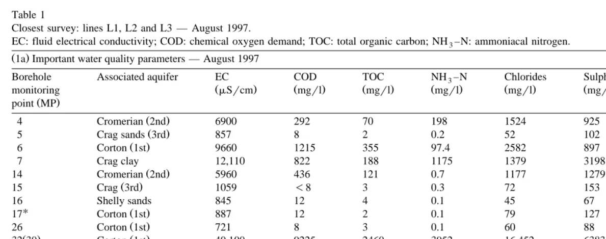
Table 1
Closest survey: lines L1, L2 and L3 — August 1997.
EC: fluid electrical conductivity; COD: chemical oxygen demand; TOC: total organic carbon; NH –N: ammoniacal nitrogen.3
Ž1a Important water quality parameters — August 1997.
Borehole Associated aquifer EC COD TOC NH –N3 Chlorides Sulphate Sodium
Ž . Ž . Ž . Ž . Ž . Ž . Ž .
monitoring mSrcm mgrl mgrl mgrl mgrl mgrl mgrl
Ž .
point MP
Ž .
4 Cromerian 2nd 6900 292 70 198 1524 925 683
Ž .
5 Crag sands 3rd 857 8 2 0.2 52 102 35
Ž .
6 Corton 1st 9660 1215 355 97.4 2582 897 1292
7 Crag clay 12,110 822 188 1175 1379 3198 944
Ž .
14 Cromerian 2nd 5960 436 121 0.7 1177 1279 298
Ž .
15 Crag 3rd 1059 -8 3 0.3 72 153 38
16 Shelly sands 845 12 4 0.1 45 67 28
U Ž .
17 Corton 1st 887 12 2 0.1 79 127 57
Ž .
26 Corton 1st 721 8 3 0.1 60 88 18
Ž . Ž .
32 30 Corton 1st 40,100 9225 2460 3952 16,452 6383 9567
Ž . Ž .
32 50 Cromerian 2nd 48,700 10,516 2308 3.873 16,327 6246 9882
Ž . Ž .
37 30 Corton 1st 1810 29 9 19.3 234 286 112
Ž . Ž .
37 50 Cromerian 2nd 2180 37 8 45.4 336 308 141
Ž .
43 Corton 1st 41,700 9806 2787 3781 11,182 8147 7727
Ž .
44 Cromerian 2nd 49,700 15,135 3350 6854 10,362 20,018 7653
Ž .
()
E.
Aristodemou,
A.
Thomas-Betts
r
Journal
of
Applied
Geophysics
44
2000
275
–
302
281
Ž1b Important water quality parameters — April 1998. Ž .
4 Cromerian 2nd 2580 84 15 52.8 327 281 174
Ž .
5 Crag sands 3rd 877 -8 1 -0.1 50 111 38
Ž .
6 Corton 1st 10,370 1103 279 85.7 2287 903 1181
7 Crag clay 39,500 4446 1268 4739 4566 13,949 3315
Ž .
14 Cromerian 2nd 6290 436 157 0.9 1108 1289 321
Ž .
15 Crag 3rd 597 41 11 0.1 41 61 21
16 Shelly sands 758 15 5 0.2 36 60 28
U Ž .
17 Corton 1st 887 12 2 0.1 79 127 57
UU
26 NrA NrA NrA NrA NrA NrA NrA NrA
UUU Ž .
32 Corton 1st 1740 205 126 34 199 105 170
UUUU Ž .
37 Corton 1st 2960 92 11 79.4 429 334 170
Ž .
43 Corton 1st 33,200 8403 1826 2385 8567 6298 5447
Ž .
44 Cromerian 2nd 15,500 3155 619 1364 1948 4764 1559
Ž .
45 Crag 3rd 939 28 10 0.1 88 88 86
U
MP17: no data available since 1997; Data shown from August 1996.
UU
MP26: no data available for April 1998.
UUU
MP32: results are reported to be an average over the whole borehole and to have been affected by high dilution due to heavy rainfall in March and April 1998.
UUUU
were detected and attributed to the disseminated metallic content of the waste.
In the past 5 years, much research has been carried out in relation to the spectral IP method and the identification of organic pollutants. This
Ž .
follows the work published by Olhoeft 1985 where the author discusses how different inter-facial processes such as the oxidation–reduction process and the clay–organic interactions may be differentiated on the basis of the observed phase spectra. Most of the work published re-cently relates to spectral IP laboratory studies
ŽVanhala et al., 1992; Boerner et al., 1993;
.
Vanhala and Soininen, 1995 where the authors use clay or sandstone samples to examine the effect of different contaminants on the complex conductivity. Field applications are reported by
Ž . Ž .
Boerner et al. 1996 and Vanhala 1997 where the authors discuss the application of the
spec-Ž .
tral IP method in a detecting organic pollu-tants in soils with both low and high clay
Ž .
particle content, and b in estimating the hy-draulic conductivity of the aquifer.
Following the above examples in the litera-ture, our research concentrated on the applica-tion of both the DC resistivity and IP methods in areas where groundwater contamination prob-lems existed and were associated with landfill waste. As the geology of the study area con-sisted of sand and clay layers, it was felt that the IP method could be a suitable method in our investigations. In addition, we were interested in investigating whether the organic contamination detected in the area through high concentrations
Ž .
of chemical oxygen demand COD and total
Ž .
organic carbon TOC would show any effect on the IP response.
Ž .
The specific objectives of our study were a the characterisation of the landfill waste in terms
Ž .
of both resistivity and chargeability, b the
Ž .
determination of the base of the landfill, c the geophysical identification of contamination in the underlying geological strata due to leachate
Ž .
movement, d the geophysical identification of clay layers in areas where these are shown to
Ž .
exist from other sources e.g., from boreholes ;
the identification of these layers is important as clay layers act as natural barriers to the down-ward movement of leachate. In addition to the above objectives, we attempted to estimate aquifer properties such as porosity and hy-draulic conductivity by combining existing mea-surements of fluid electrical conductivity with the geophysical inversion results.
2. Geological setting and site description
Our area of investigation lies in East Anglia, UK, where the geological setting consists of alternating layers of clay and sand of variable thickness. The sediments within the depth of interest are of Quaternary marine and glacial origin, overlying the London clay, which occurs at approximately 70 m depth. At greater depths, the London clay is believed to overlie a Chalk formation. Past geological studies show that the aquifer system consists of a sequence of three
Ž .
sand aquifers top, middle, and bottom , with intervening semi-pervious clay aquitards
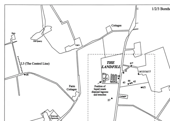
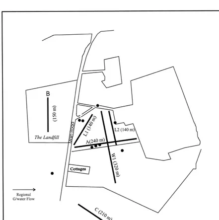
ŽRichardson, 1996 . A map of the area together.
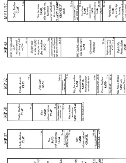
with the boreholes of interest and the up-gradi-ent geophysical control line is shown in Fig. 1. The plan view of the landfill with its lagoons and trenches can also be seen in this figure. The detailed individual borehole logs are shown in Fig. 2. From these, it is observed that the thick-ness of both the top and middle aquifers is variable throughout our study area. From the log of borehole MP32, the first sand aquifer lies at a depth between 7 and ;16.4 m, while the first semi-pervious silty sandrclay aquitard ap-pears between 16.4 and ;18.0 m. For borehole MP14r15r16r17, the first aquitard appears at ;20 m depth with the top aquifer lying be-tween 5.5 and 20 m. For borehole MP43, there seems to be no aquitard in the first ;29 m and
Ž
top and middle aquifers Corton and Cromerian
.
sands appear as one unit. In all cases, there is a
Ž .
thick top layer overburden of boulder clay whose thickness also varies from location to
Ž .
( )
E. Aristodemou, A. Thomas-BettsrJournal of Applied Geophysics 44 2000 275–302 283
Ž .
and 11.0 m borehole MP 37 . There are no logs for boreholes MP4r5 and MP 6r7.
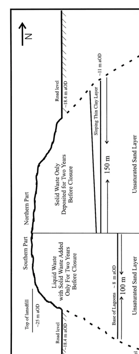
A schematic of a vertical cross-section along the central part of the landfill, from south to north, is given in Fig. 3. The site forms a small hill with its highest region approximately 7 m
Ž
above surrounding ground level ;25 m above
.
ordnance datum, OD and with a flat region at
the top approximately 150 m long. The water level is approximately ;23.5 m below the top
Ž
flat region of the landfill equivalent to ;1.5 m
.
above OD . The natural clay base of the landfill in the northern part of the site is ;14 m from
Ž .
the top ;11 m above OD while the base of the excavated trenches and lagoons in the
south-Ž
ern site was ;17 m from the top ;8 m above
.
OD . The landfill was set in operation in the 1950s after the closure of a clay pit used for brick making. Initially, the waste deposited was of domestic nature and it was placed in the south-western part of the present site. However, in the early 1970s, the deposition of liquid waste began lasting up to 1989 when the opera-tion of the site was terminated. The site re-ceived both oily and non-oily waste with two of its lagoons, B1r2 and B3 in Fig. 1, receiving the liquid waste. These lagoons had a natural
Ž .
clay base, while lagoon A also Fig. 1 and the existing trenches had no clay base at all, but were excavated straight into the underlying sand layer. From the limited information available on the type of waste deposited, it appears that 65–80% of the waste was agrochemical with solvents, ammonia, and heavy metals being de-posited in small but consistent quantities. There was also regular disposal of mercury and cop-per, as well as of a number of volatile organic carbons and phenolic compounds.
As indicated in the vertical cross-section in Fig. 3, the liquid waste was disposed in the southern part of the site. However, 2 years before the closure of the site, a co-disposal operation was set-up with solid waste being
deposited in both the southern and northern parts of the site. An inclined natural clay base
Ž
was left in the northern part ;11 m above
.
OD so that any accumulation of leachate would naturally drain into the lagoons in the southern part. The main reason for introducing solid waste to the site was to effect a reduction of a hy-draulic mound that developed underneath the landfill, due to the deposition of the liquid waste. This hydraulic mound affected the local groundwater flow movement and resulted in its reversal. Hydrogeological studies carried out since the closure of the site in 1989 indicate the elimination of this hydraulic mound and the local groundwater flow direction following the
Ž .
regional one Bartlett and Dottridge, 1996 . A substantial amount of water quality infor-mation data exists from the boreholes dis-tributed around the site with clear indications of contamination of both the top and middle aquifers in the eastern part of the site. Water samples have been taken on a quarterly basis for a number of years by the landfill operators and have been analysed for both organic
contamina-Ž .
tion parameters COD, TOC and inorganic
pa-Ž
rameters chlorides, sulphates, ammoniacal
ni-Ž ..
trogen NH –N3 as well as heavy metals and
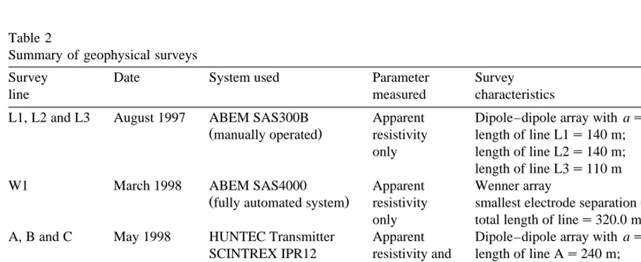
Table 2
Summary of geophysical surveys
Survey Date System used Parameter Survey
line measured characteristics
L1, L2 and L3 August 1997 ABEM SAS300B Apparent Dipole–dipole array with as5 m;
Žmanually operated. resistivity length of line L1s140 m; only length of line L2s140 m; length of line L3s110 m
W1 March 1998 ABEM SAS4000 Apparent Wenner array
Žfully automated system. resistivity smallest electrode separations4.0 m; only total length of lines320.0 m A, B and C May 1998 HUNTEC Transmitter Apparent Dipole–dipole array with as15.0 m;
SCINTREX IPR12 resistivity and length of line As240 m; receiver chargeability length of line Bs150.0 m;
length of line Cs210.0 m Soundings S1 May 1998 HUNTEC Transmitter Apparent Schlumberger array
and S2 SCINTREX IPR12 resistivity and total length of soundings150.0 m
( )
E. Aristodemou, A. Thomas-BettsrJournal of Applied Geophysics 44 2000 275–302 285
electrical conductivity. The borehole log infor-mation together with the water level and fluid conductivity measurements at these locations are used in the interpretation of the geophysical results. An example of the concentration values of the most important parameters measured at the different monitoring points in August 1997
is given in Table 1a. As can be seen high concentrations of chlorides, sulphates, NH –N3
and sodium ions as well as of COD and TOC are recorded at boreholes MP32, MP43 and MP44 being indicative of contamination in both the top and middle aquifers. Similar contamina-tion levels are observed in April 1998 as shown
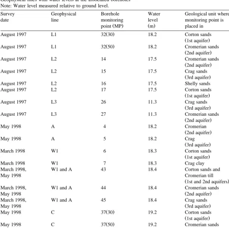
Table 3
Geophysical lines with water levels at the associated boreholes Note: Water level measured relative to ground level.
Survey Geophysical Borehole Water Geological unit where
date line monitoring level monitoring point is
Ž . Ž .
point MP m placed in
Ž .
August 1997 L1 32 30 18.2 Corton sands
Ž1st aquifer. Ž .
August 1997 L1 32 50 18.2 Cromerian sands
Ž2nd aquifer.
August 1997 L2 14 17.5 Cromerian sands
Ž2nd aquifer.
August 1997 L2 15 17.5 Crag sands
Ž3rd aquifer.
August 1997 L2 16 17.5 Shelly sands
August 1997 L2 17 17.5 Corton sands
Ž1st aquifer.
August 1997 L3 26 11.3 Crag sands
Ž3rd aquifer.
August 1997 L3 27 11.3 Cromerian sands
Ž2nd aquifer.
May 1998 A 4 18.2 Cromerian
Ž2nd aquifer.
May 1998 A 5 18.2 Crag
Ž3rd aquifer.
March 1998 W1 6 18.3 Corton sands
Ž1st aquifer.
March 1998 W1 7 18.3 Crag clay
March 1998, W1 and A 43 18.4 Corton sands and
May 1998 Cromerian till
Ž1st and 2nd aquifers.
March 1998, W1 and A 44 18.4 Cromerian sands
Ž .
May 1998 2nd aquifer
March 1998, W1 and A 45 18.4 Crag sands
Ž .
May 1998 3rd aquifer
Ž .
May 1998 C 37 30 19.2 Corton sands
Ž1st aquifer. Ž .
May 1998 C 37 50 19.2 Cromerian sands
Ž2nd aquifer.
May 1998 Sounding 32 18.2 Corton and Cromerian sands
Ž .
S1 1st and 2nd aquifer
May 1998 Sounding 43 and 44 18.4 Corton and Cromerian sands
Ž .
in Table 1b, with the exception of MP32. This, according to site operators, is most likely due to high dilution effects in an unreliable borehole. Borehole MP44 also shows a considerable con-trast between the two surveys dates.
3. Geophysical data acquisition
Geophysical lines were set-up as close to monitoring boreholes as possible within the lo-gistical constraints. Both profile and sounding data were collected at the site over a period of 2
Ž .
years 1997–1998 . As groundwater is known to be moving towards the east our investigation was concentrated east of the landfill with the
Ž .
exception of the control line L3 see Fig. 1 . Fig. 4 shows the landfill in relation to the investigations lines and the sounding centres as well as the boreholes of interest. Hedges, houses, and roads are also shown in order to emphasise the obstacles encountered during the surveys which restricted the lengths of some of our survey lines, thus, limiting the depth of investi-gation. Line B was right on the top of the landfill where a flat region existed allowing a maximum length of 150 m. Schlumberger sounding measurements were taken at only two centres. All profile data were collected using the dipole–dipole configuration with the exception of the W1 line, where the Wenner array was used. The surveys were carried out with a vari-ety of field equipment which had an effect on both the quantity and quality of the data col-lected. The length of the lines surveyed, the data acquisition systems used and the parameters measured are summarised in Table 2 while Table 3 shows the geophysical lines in relation to their nearest monitoring points. The water levels measured at these points are also shown.
4. Data analysis
The apparent resistivity and chargeability measurements, with the exception of profile W1,
were inverted using the two dimensional com-mercial software DCIP2D — a resistivity and IP inversion software based on the work by
Ž .
Oldenburg et al. 1993 and Oldenburg and Li
Ž1994 . The Wenner resistivity data from profile.
W1 were inverted using the RES2DINV
soft-Ž .
ware Loke and Barker, 1996 . The inversion approaches are explained in detail in the DCIP2D and RES2DINV manuals and in the above mentioned papers and therefore the com-plexities of inversion algorithms will not be discussed here. It suffices to note that the goal of a resistivityrchargeability inversion algo-rithm is to recover a physically realistic set of model parameters that adequately reproduces the given set of field observations. To overcome the problem of non-uniqueness, an objective function is defined which when minimised pro-duces a model that follows certain character-istics as specified by the user as well as result-ing in a model response that has a good fit to the measured data. For example, in the DCIP2D software, the user can specify how smooth the final model should be in a given direction by choosing appropriate values of the smoothing parameters and can specify how close to a given reference model the final model should be. The fit between the measured data and the model response is assessed through the chi-square mis-fit function.
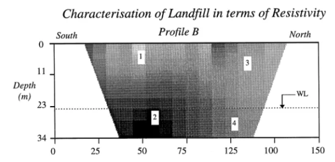
5. Interpretation of results
( )
E. Aristodemou, A. Thomas-BettsrJournal of Applied Geophysics 44 2000 275–302 287
Fig. 5. Characterisation of the landfill in terms of resistivity.
5.1. Landfill characterisation
Ž .
The inversion results along line B Fig. 4 are shown in Figs. 5 and 6, respectively. In the final resistivity inversion model, three different zones can be distinguished. The low resistivities within the landfill in Zone 1 are believed to be associ-ated with both the liquid and solid waste. These are also consistent with the high concentrations of inorganic material recorded in the boreholes
Ž .
within the site e.g., borehole MP38 . Zone 2 has lower resistivities between 11 and 23 m depth and even lower values at depths below 23 m. One possible explanation for the lower val-ues is the natural clay base that exists below
some of the lagoons. Alternatively, they could be attributed to the accumulation of leachate and the contamination of the saturated sand, especially since lagoon A and the trenches were excavated into the underlying sands. The latter explanation is favoured as the water table is recorded at ;23.5 m from the top of the landfill. Zone 3 corresponds to the northern part of the landfill, most likely representing the ;14 m thick unconsolidated solid waste which was deposited in the last 2 years of operation of the landfill. In this zone, we observe similar resis-tivities as in Zone 1. From the schematic of the
Ž .
landfill Fig. 3 , a thin sloping clay layer exists on the northern side at ;14 m depth from the
top of the landfill, which is intended to drain any formed leachate into the southern part. This would explain the marked resistivity contrast between the north and south sections with the higher resistivities observed in Zone 4 than in
Ž
Zone 2 in the saturated sections i.e., below the
.
water table .
The chargeability lateral variations along the profile are small. However, throughout the sec-tion the values are high, indicating the presence of the landfill, and ranging between 80 and 120 ms. Zones 1 and 3 show chargeabilities in the lower end of the range while Zones 1 and 4 are in the upper end. The higher chargeabilities in Zones 1 and 4 may be due to higher concentra-tions of liquid waste andror an increase in metallic waste content. In particular, the in-creased chargeabilities in Zone 4 correlate with the saturated zone where, as the resistivity re-sults suggest, contamination due to the accumu-lation of leachate is believed to be occurring.
Combining resistivity and chargeability con-trasts, we may conclude that the following.
Ž .i It was possible to distinguish between the upper unsaturated and the lower saturated fill and hence the contaminated water table at ;23 m below the top of the landfill in the southern part of the site. Substantial lowering of resistivi-ties and increase of chargeabiliresistivi-ties are observed at this depth which is believed to be due to the contamination of groundwater by the accumula-tion of leachate.
Ž .ii Although low resistivities are also ob-served in the northern part of the profile there does not seem to be a clear contrast at the expected water level; two possible reasons for this, affecting the total amount of leachate
avail-Ž .
able in the northern part of the site, may be a the fact that only solid waste is deposited in the northern part and therefore less leachate is
pro-Ž .
duced b the presence of the inclined clay base draining any leachate from the north to the south.
Ž .iii Due to the high concentrations of leachate, it was not possible to identify the inclined clay base in the northern part of the site
nor the clay base of some of the lagoons in the southern part.
5.2. The control line L3
Ž .
A survey L3 was carried out well away from the site and to the west of it to act as a control. At this location, we expected no con-tamination as groundwater is moving eastwards
Ždown-gradient . The nearest borehole to the.
up-gradient survey profile L3 was borehole MP26, shown in Fig. 1. According to the bore-hole log, the boulder clay is very thin at this
Ž .
location ;0.5 m thick compared to the other locations east of the landfill. Thus, our geophys-ical measurements are representative of the first sand aquifer without the conductive overburden. The water table recorded at borehole MP26 is around 11.3 m, while the measured fluid con-ductivity has the low value of 721 mSrcm which is considered as the background, uncon-taminated value.
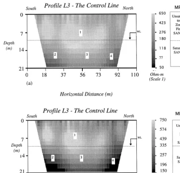
The resistivity model obtained for this profile is shown in Fig. 7. From the results, three zones were identified. Zone 1 represents the unsatu-rated zone above the recorded water table and it is a highly resistive zone with resistivity values exceeding 550 V m. For the first ;70 m of the profile, Zone 2 corresponds to the saturated
Ž .
aquifer at depths below the water table 11.3 m and its lower resistivities in the range of 150– 550 V m reflect this. Zone 3, between 70 and 110 m along the profile, corresponds to the resistive zone that extends below the expected water table. This may be due to lower porosities in this part of the profile, which would imply lower fluid content and therefore increased bulk resistivities.
5.3. Profiles L1 and L2 — the unsaturated zone
The first two profiles to be considered east of the landfill are profiles L1 and L2, surveyed in August 1997. The boreholes associated with them are boreholes MP32 and MP14r15r
Ž .
( )
E. Aristodemou, A. Thomas-BettsrJournal of Applied Geophysics 44 2000 275–302 289
Ž
Fig. 7. Resistivity inversion model for the control line L3 same results, on two plot scales, for ease of comparison with Figs.
.
8, 9, 11 and 12 .
data shown in Table 3, the average water level measured at these boreholes was ;18.0 m. The lengths of L1 and L2 were limited to 150 m due to restrictions in space thus allowing a maxi-mum depth of investigation of ;20 m. Consid-ering lines L1 and L2, we could therefore only assess geophysically the unsaturated zone down to ;18 m depth. It was not possible to draw any conclusions in relation to the contamination in the saturated zone, as data in this zone were
Ž
very limited only two to three meters of
infor-.
mation . The final inversion models for L1 and L2 are shown in Figs. 8 and 9, respectively.
Fig. 8. Resistivity inversion model for line L1.
line are so high that the explanations associated with contamination are favoured. Zone 3 is very resistive with resistivities approaching those of line L3. Thus, it is believed that this section is unaffected by contamination.
Ž .
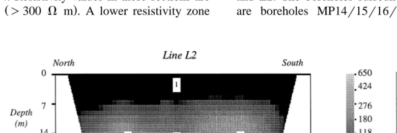
For profile L2 Fig. 9 , the conductive clay
Ž .
overburden is again identified Zone 1 , but as in profile L1, since the information for depths greater than 18 m was very limited, no final conclusions could be made with regards to the contamination in the saturated zone of the top aquifer. Resistive zones for the depth range between 14 and 21 m are identified for the lengths along the profile between 20 and ;60 m and between 75 and 121 m, denoted as Zones 2 and 4. Resistivity values in these sections are
Ž .
higher )300 V m . A lower resistivity zone
Ž-276 V m , denoted as Zone 3, is also identi-.
fied between 60 and 75 m for depths greater than 18 m, which could be an indication of contamination although not conclusively.
5.4. Identification of contamination in the satu-rated zone
5.4.1. Profile W1
As no decisive conclusions on the contamina-tion in the saturated aquifers could be made from the results of profiles L1 and L2, due to their limited lengths, further measurements were needed. Additional data were taken along a much longer line W1, which lay between L1 and L2. The boreholes surrounding this profile
Ž .
are boreholes MP14r15r16r17 eastwards ,
( )
E. Aristodemou, A. Thomas-BettsrJournal of Applied Geophysics 44 2000 275–302 291
Ž .
borehole MP6r7 in the north and borehole
Ž .
MP44 west . The automated ABEM SAS400 instrument was used in this case with the Wen-ner array. The length of the line was 320 m, thus, allowing a greater lateral coverage for depths up to 50 m. Thus, information on both
Ž .
the top aquifer down to ;20 m depth and
Ž .
middle aquifer down to ;28 m depth could be obtained.
The measurements as well as the inversion results for this profile are shown in Fig. 10. Looking at the resistivity inversion model along the whole profile, four resistivity zones could be distinguished. Zone 1 represents the conductive
Ž .
overburden -75 V m for the whole length of the profile, in agreement with borehole informa-tion which indicates a thick boulder clay top layer. Zone 2 is a more resistive zone with resistivities greater than 200 V m while Zones
Ž .
3 and 4 are more conductive -200 V m . Bearing in mind that the regional groundwa-ter flow is eastwards, the lower resistivities found in Zones 3 and 4, for depths greater than ;17 m, may be indicative of an eastward movement of contamination from the landfill.
Ž .
Although the information from line L2 Fig. 9 was depth limited to ;20 m, the lower
resistiv-Ž .
ities in its Zone 3 Fig. 9 seems to be consis-tent with the lower resistivities found in Zone 3
Ž .
of the profile W1 Fig. 10 .
Two more profiles, profiles A and C, were carried out in order to investigate the southward movement of any contamination as the water samples from boreholes MP43 and MP44
indi-Ž .
cated high fluid conductivities Table 1a and b . Profile A will be discussed first.
5.4.2. Profile A
Both resistivity and chargeability measure-ments were taken along this profile whose total length was 240 m, thus, allowing a depth of investigation down to ;30 m covering both the top and middle aquifers. According to the
bore-Ž
hole information along this profile boreholes
.
MP43 and MP44 , the first aquitard is non-ex-istent and the two aquifers in fact form one unit.
The resistivity and chargeability inversion mod-els for line A are shown in Fig. 11a and b, respectively.
5.4.2.1. ResistiÕity model. Four zones are identi-fied in the resistivity model, with Zone 1 repre-senting the conductive overburden and the un-saturated zone down to the depth of 17 m. Zone 2 is a resistive zone, while Zone 3 is a lower resistivity region which is thought to be associ-ated with the contamination plume. Zone 4 is a highly resistive section between 160 and 200 m with resistivities greater than 550 V m.
5.4.2.2. Chargeability model. Three chargeabil-ity zones are identified in the chargeabilchargeabil-ity model. Zone 1 is a low chargeability zone along the whole length of the profile with chargeabili-ties -5 ms, while Zone 2 has higher charge-ability values in the western part of the profile, between 80 and 120 m, and for depths greater than 17 m. These higher chargeability values correspond to the lower resistivity Zone 3 of the resistivity model and could be an indication of contamination. Zone 3 is a low chargeability region associated with the high resistivity Zone
Ž .
4 of the resistivity model Fig. 11a .
Ž .
Comparing i the fluid conductivity values
Ž .
in the boreholes close to line A, ii the bulk resistivity values obtained from the resistivity
Ž .
inversion and iii the chargeability model re-sults, we observe that although the fluid resistiv-ities are very low in the first and second aquifers
Žrw;0.3 and 0.65 V m, respectively; Table
.
( )
E. Aristodemou, A. Thomas-BettsrJournal of Applied Geophysics 44 2000 275–302 293
Ž . Ž .
Fig. 11. a Resistivity inversion model for profile A. b Chargeability inversion model for profile A.
Ž .
ability model Zone 2 where high
chargeabili-Ž .
ties exist up to 20 ms which cannot be due to the presence of clay particles as the
chargeabil-Ž .
ity values due to clay are lower -10 ms . These higher chargeabilities in the western part of the profile may therefore be related to the presence of the organic waste detected in the boreholes.
A second possible explanation of the low fluid resistivities and high bulk resistivities may be related to the pore geometry itself as
dis-Ž .
cussed by Herrick and Kennedy 1994 . Accord-ing to these authors, in a given pore system, pore throats exhibit high current densities while the nearly stagnant volumes in isolated parts of the pore system exhibit low current densities. This non-uniform current density distribution caused by the pore geometry may affect the overall electrical efficiency of the rock.
5.4.3. Profile C
In order to establish the southern boundary of a contamination ‘plume’, we also looked at both the resistivity and chargeability inversion results along line C, shown in Fig. 12a and b, respec-tively. The closest boreholes to this profile are MP37 in the NW end of the profile, MP43 in the central region, and MP4r5 in the SE end of the profile. All three boreholes show fluid elec-trical conductivities above the background,
un-Ž .
contaminated value Table 1a and b . The resis-tivity inversion model is shown in Fig. 12a where we can distinguish four zones.
5.4.3.1. ResistiÕity model. Although there is a lateral variation of resistivities along the profile,
Ž
it is only in the very early part for the length of
.
Ž . Ž .
Fig. 12. a Resistivity inversion model for profile C. b Chargeability inversion model for profile C.
m. This is represented by Zone 3 in Fig. 12a and the resistivities observed are similar in val-ues to the ones found in Zone 3 of profile A
ŽFig. 11a . These resistivities could be an indi-.
cation of the presence of contamination and in particular of inorganic waste. However, as our line is ;200 m away from the borehole MP4r5, it is yet unclear as to whether this is the case. Also, the low resistivities in Zone 3 of profile A were associated with high chargeabili-ties. There is no such correlation between resis-tivity and chargeability values for the resisresis-tivity
Ž .
Zone 3 of profile C Fig. 12a and b .
For the rest of the profile and at depths between 17 and 30 m, the resistivities are greater than 300 V m. The thick highly resistive zone
Ž .
in the latter part of the profile )140 m for the depths between 17 and 33 m has resistivities greater than 500 V m while as we move to-wards the centre of the profile there is a ‘thin-ning’ of this resistive zone with resistivities ranging between 300 and 500 V m.
5.4.3.2. Chargeability model. The chargeability
Ž .
model corresponding to this profile Fig. 12b shows a layered structure with chargeabilities increasing uniformly with depth. Such a uni-formly layered chargeability inversion model would appear to suggest that at least no organic waste has reached this part. The low
chargeabil-Ž .
( )
E. Aristodemou, A. Thomas-BettsrJournal of Applied Geophysics 44 2000 275–302 295
the boreholes east of the landfill, while the high chargeabilities at ;30 m depth may be related to the semi-pervious clay layer, also found in the surrounding boreholes. The observed differ-ences in chargeabilities between the two layers of clay may be diagnostic of different composi-tions.
Comparing the resistivity and chargeability results, it is unclear as to whether the lateral variations in resistivity are associated with any contamination. The chargeability model showed no lateral variations, thus, no link to inorganic or organic contamination could be made as was the case for line A.
Following the above individual description of the results, the output from four ‘parallel’ lines has been displayed in Fig. 13. This shows the variation of resistivities east of the control line L3, and leads us to suggest that the movement of contamination is not only towards the east, but also towards the SE direction.
5.5. Schlumberger soundings
In addition to the 2D measurements using the dipole–dipole and Wenner arrays, we also car-ried out Schlumberger soundings at two loca-tions, S1 near borehole MP32 and S2 near borehole MP43. Resistivity data were collected to see whether we could resolve the parameters of the different layers, especially their resistivi-ties. Of special interest was the resolution of the clay layer identified in the borehole close to
Ž .
sounding S1 borehole MP32 . The apparent resistivity data were inverted using the 1D
in-Ž .
version program of Sandberg 1990 . During the inversion procedure, the borehole log informa-tion enabled us to constrain the thickness of the layers.
For sounding S1, the water sampling
infor-Ž .
mation from borehole MP32 Table 1a showed high levels of contamination within both the top and middle aquifers. The apparent resistivity
curve seen in Fig. 14 seems more suited to a two-layer case than a five-layer case as indi-cated by the borehole log. However, the starting model for the inversion represented the layered structure according to the borehole log with three layers over a half space where the half-space corresponded to the middle aquifer. Dur-ing the inversion, all depths were constrained. The results are shown in Fig. 14 together with the final models, as well as the log of borehole MP32. The comparison between model re-sponse and real measurements show a very good fit to the data and the parameter values obtained are physically realistic. However, the
Ž
parameter resolution information see Sandberg,
.
1990 associated with the final model showed the resistivity of the third layer, corresponding to the thin clay layer, was not resolved.
At the second location, the clay layer is non-existent according to the borehole log for MP43. The apparent resistivity curve at this centre also resembles more of a two-layer case. The starting model used during the inversion
consisted of three layers over a half space and all depths were constrained again according to the borehole information. The inversion results together with the final inversion model are shown in Fig. 15. Again, although a good fit to the data was obtained, the resistivities of the third layer and of the half-space were not re-solved.
It is important to note that in isolated Schlumberger soundings only 1D inversion is possible, whereas the subsurface distribution of resistivities, contributing to the measured appar-ent resistivities may be 2D or 3D. It is therefore not surprising that the model parameters cannot be resolved.
In these 1D inversions, we also observe the relatively high resistivities obtained for the lay-ers representing the aquiflay-ers, especially in sounding S2. Despite the fact that the fluid conductivity and chloride levels are very high at these locations, the bulk resistivity is very high
Ž .
for sounding S2 862 V m . The high resistivity values obtained in regions where the fluid
( )
E. Aristodemou, A. Thomas-BettsrJournal of Applied Geophysics 44 2000 275–302 297
Fig. 15. Schlumberger sounding S2 — measurements, predictions and resistivity model.
Ž .
tivity is low high conductivity is not what is expected and as explained earlier these high bulk resistivities could be associated with the presence of organic contamination parameters
Žhigh concentrations of COD and TOC
indi-.
cated by borehole MP43 or alternatively with the low porosity and pore geometry. Addition-ally, it needs to be borne in mind that the distortions introduced by treating a 3D problem with 1D or 2D modelling procedures can be quite significant and may produce a bias to-wards the high resistivity values.
6. Determination of aquifer properties
In order to obtain quantitative answers in groundwater flow and contaminant transport modelling, it is essential to have estimates for the hydraulic properties of any given aquifer system such as the hydraulic permeability and conductivity. Such values are usually obtained either from pumping tests or laboratory experi-ments when core samples exist. However, an alternative approach can be applied, which
utilises non-invasive geophysical information. Geophysicists have realised for some time that a correlation between the hydraulic and electrical properties of an aquifer should be possible, as both these properties relate to the pore space
Ž
structure and heterogeneity Kelly, 1977; Mazac et al., 1985; Huntley, 1986; Mazac et al., 1988; Boerner et al., 1996; Christensen and Sorensen,
.
1998 . The diversity of the relationships re-ported indicates the complexity of the problem, with all authors emphasising the fact that these relationships are specific to the site under inves-tigation.
Since we had bulk and fluid resistivities at several locations, it was desirable to see if it was possible to obtain hydraulic conductivity values using the Kozeny–Carman–Bear
equa-Ž .
6.1. Determination of porosity through the in-trinsic formation factor Fi
Archie’s law relates the bulk resistivity of a fully saturated granular medium to its porosity and the resistivity of the fluid within the pores
Ž .
according to Eq. 1 .
r sar fym
Ž .
1o w
where ro is the bulk resistivity, rw is the fluid resistivity, f is the porosity of the medium and m is known as the cementation factor, although it is also interpreted as grain-shape or pore-shape factor; the coefficient a is associated with the medium and its value in many cases departs from the commonly assumed value of one. For a clay-free, clean medium, the ratio rorrw is known as the intrinsic formation factor F .i
The values of the coefficients a and m should, ideally, be determined for each site under inves-tigation. However, due to lack of core samples in our test area, this was not possible and an alternative approach was adopted whereby a wide range of values for a and m reported in the literature was used to obtain porosity
esti-Ž .
mates. Worthington 1993 reports three differ-ent expressions for the intrinsic formation factor in relation to the porosity associated with sam-ples from different locations. We use these three relationships to estimate the porosity, as well as a fourth expression in which the coefficient a has the value of one while m is allowed to vary
Ž
between 1.3 and 2.5 Jackson et al., 1978; de
.
Lima and Sharma, 1990 .
The first step in our procedure to estimate the hydraulic conductivity is the determination of the intrinsic formation factor F from whichi
Ž .
porosity can be estimated via Eq. 1 for differ-ent values of a and m. However, for field data a complication arises due to the fact that Archie’s
Ž Ž ..
formula Eq. 1 is valid only for clay-free, clean, consolidated sediments. Any deviations from these assumptions make the equation
in-Ž .
valid as discussed by Worthington 1993 . In
the case of unclean, clayey sands the ratio of bulk resistivity to fluid resistivity is known as the apparent formation factor F . As our aquifera system consisted of clayeyrsilty sand material, a modified representation of the Archie’s equa-tion was required. For this reason, the
Wax-Ž
man–Smits model was considered Vinegar and
.
Waxman, 1984 which relates the apparent and intrinsic formation factors F and F after tak-a i
ing into account shale effects. According to
Ž .
Worthington 1993 ,
y1
FasF 1i
Ž
qBQvrw.
Ž .
2where the BQv term relates to the effects of surface conduction, mainly due to clay particles. When the surface conduction effects are non-ex-istent, then the apparent formation factor is equal to the intrinsic one, i.e., FasF .i
Ž .
Re-arranging the terms of Eq. 2 , we obtain a linear relationship between 1rF anda rw,
1rFas1rFiq
Ž
BQvrFi.
rwŽ .
3where 1rF is the intercept of the straight linei
Ž
and BQvrF represents the gradient Huntley,i
.
1986; Worthington, 1993 . Thus, by plotting 1rFa vs. fluid resistivity rw, we should, in principle, obtain a value for the intrinsic forma-tion factor, which will subsequently enable us to estimate porosity.
To follow the above approach, we used bulk resistivities ro from our resistivity inversion results together with the fluid electrical resistivi-ties rw at the nearest boreholes, to obtain values of the apparent formation factor Fasrorrw for
Ž .
the saturated top aquifer. From Eq. 3 , it is clear that a major source of error would be the wrong estimation of the apparent formation fac-tor which depends on the bulk resistivity as obtained from the inversion models. Thus, as-suming the fluid resistivities were measured correctly in the laboratory, we considered by how much the bulk resistivities from the inver-sions could vary. This uncertainty was mainly
Ž
( )
E. Aristodemou, A. Thomas-BettsrJournal of Applied Geophysics 44 2000 275–302 299
Table 4
Estimating apparent formation factor from the geophysical data top aquifer
MP Associated Depth Fluid EC rw r0 Fa 1rFa
Ž . Ž . Ž . Ž .
line m mSrcm Vm Vm
Ž .
6 W1 19.3 10,370 April 1998 0.96 89.1 92.8 0.0108
Ž .
6 W1 19.3 10,370 April 1998 0.96 129.7 135.1 0.0074
Ž .
37 C 20.1 3875 April 1998 3.38 198 58.6 0.017
Ž .
37 C 20.1 3875 April 1998 3.38 296 87.6 0.011
Ž .
26 L3 12.3 721 August 1997 13.8 432 31.30 0.0319
Ž .
26 L3 12.3 721 August 1997 13.8 530 38.41 0.0260
.
borehole MP37, line C , were at some distance away from the region represented in the resistiv-ity model. To obtain a measure of the uncer-tainty, we considered average bulk resistivities over stretches of the survey lines, thus, enabling estimates of the upper and lower limits of the bulk resistivity value ro for the lines L3, C and W1.
The resistivity values obtained from the in-versions, after averaging to allow for lateral variations along each profile, and the estimated apparent formation factors are shown in Table 4. Fig. 16 shows 1rF plotted against the fluida
resistivity rw and the best fit straight line gives the inverse of the intrinsic formation factor Fi
which for our data set was 0.0083. The
porosi-Fig. 16. 1rF vs. fluid resistivitya rw.
Ž .
ties could now be determined through Eq. 1 for reported values of a and m for sands as shown in Table 5.
6.2. Determination of hydraulic conductiÕity
The estimation of the hydraulic conductivity was achieved through the use of the Kozeny– Carman–Bear equation, given by Domenico and
Ž .
Schwartz 1990 as:
2 3 2
Ks
Ž
dvgrm.
Ž
d r180.
f rŽ
1yf.
Ž .
4where d is the grain size, dv is the fluid density
Ž 3.
taken to be 1000 kgrm , and m is the
dy-Table 5
Sensitivity analysis on porosity and hydraulic conductivity estimates
Porosity estimates using different Archie’s coefficients
Ž1rFis0.0083 , together with the sensitivity analysis in-.
vestigating the effect of porosity on hydraulic conductivity.
Ž
Intrinsic formation factor Fis0.0083. Grain sizes0.4
.
mm.
a m Porosity Hydraulic
Ž .
conductivity mrs
1.04 2.3 0.127 1.28Ey05
0.5 2.31 0.093 5.05Ey06
1.1 1.61 0.054 9.87Ey07
1 1.3 0.025 9.82Ey08
1 1.5 0.041 4.29Ey07
1 1.7 0.059 1.33Ey06
1 1.9 0.080 3.24Ey06
1 2.1 0.102 6.69Ey06
1 2.3 0.125 1.22Ey05
namic viscosity taken to be 0.0014 kgrms
ŽFetter, 1994 . The reported values for the grain. Ž
size range between 0.2 and 0.6 mm
Richard-.
son, 1996 . In our estimations, we assumed at this stage a mean particle size of 0.4 mm consis-tent with exposures on the coastal section. The
Ž .
hydraulic conductivity values using Eq. 4 are shown in Table 5.
The reported geometrical mean hydraulic conductivity value for this aquifer is 9.3Ey7 mrs while the corrected geometrical mean value
Ž .
becomes 4.4Ey06 mrs Richardson, 1996 . Looking at Table 5, we can see that the low porosity values within the range of 0.05–0.10
Žbased on as1 and m ranging between 1.5 and
.
2.1 result in hydraulic conductivity values of the same order of magnitude as the ones
re-Ž .
ported by Richardson 1996 .
In comparing these values, it is important to bear in mind that the physical measurements are made in small samples and a limited zone around the borehole, whereas the geophysical methods use properties averaged over large volumes.
7. Summary and conclusions
By applying the geo-electrical methods, we have been able to characterise the landfill in terms of resistivity and chargeability and distin-guish between the southern and northern sec-tions, which received different types of waste. A more contaminated saturated zone in the south-ern part could be distinguished, which is be-lieved to be due to the accumulation of leachate, mainly from the deposited liquid waste. Using the chargeability inversion results we were also able to distinguish the zone below the water table within the landfill.
In addition, we were able to follow the east-wards movement of contamination by compar-ing the resistivity results from lines L1, L2 and W1 to the control line L3. Resistivity contrasts are observed in lines L1 and W1, suggesting
inorganic contamination as detected in the nearby boreholes. Lateral resistivity contrasts along line L2 are less obvious, with only a small central section shown to be affected by contamination.
Lines A and C were investigated in the at-tempt to establish the southern boundary of the contamination. Both resistivity and chargeabil-ity results were available on these lines. Line A shows resistivity contrasts that may be related to contamination, while with profile C the effects of contamination are not obvious. On profile A, there is a marked difference in the chargeability values within the saturated zone, with the in-creased chargeability values in the western part of the profile suggesting the presence of organic contamination. On the contrary, the results for profile C show no lateral variations, but rather a uniformly layered chargeability model with chargeabilities increasing with depth up to the second clay aquitard at ;28 m depth. From the results of these two profiles, it is clear that IP information helped to distinguish more clearly regions affected by contamination.
An intriguing general observation is that the bulk resistivities obtained from the inversions
Žwhether 2D or 1D are quite high 200–300. Ž V
.
m . This happens in regions where contamina-tion is known to exist from the low fluid resis-tivity measurements in the nearby boreholes
Ž;0.3 V m . With such low fluid resistivities.
one would expect the bulk resistivities also to
Ž .
be low -50 V m . One possible explanation for the unexpectedly high bulk resistivities may be the presence of organic pollutants since bore-hole fluids show high concentrations of parame-ters such as COD and TOC, in addition to the inorganic pollutants. The precise mechanism for this is not clear however and further study is needed; indeed lowering of resistivities by bac-terial action on organics has also been reported
Ž .
in the literature e.g., Benson et al., 1991 . An alternative explanation for the high bulk resis-tivities is low porosity values and the pore geometry itself, as discussed by Herrick and
Ž .
( )
E. Aristodemou, A. Thomas-BettsrJournal of Applied Geophysics 44 2000 275–302 301
electrical efficiency of the system. An addi-tional factor to be taken into account in future studies of this area may be the distortion effects of a 3D problem on the 1D and 2D solutions. To eliminate these effects, a 3D data set would be required, which would inevitably increase the survey time and costs.
Using the bulk resistivities from the inver-sions, the measured fluid resistivities and the intrinsic formation factor derived from them, an attempt was made to estimate a range of poros-ity values for the top aquifer, using reported values for the parameters in the empirical Archie’s formula. These porosities were subse-quently used to estimate the hydraulic conduc-tivity through the Kozeny–Carman–Bear equa-tion. A range of porosity values was established for which the hydraulic conductivity estimates cluster well and fall within an order of magni-tude of values reported from other sources. Given the nature and extent of uncertainties, it is encouraging that this degree of agreement exists between the geophysically based values and the other methods, and it is reasonable to conclude that geophysical estimates, at the very least, provide a useful additional constraint on the hydraulic conductivity values.
Acknowledgements
We would like to thank the reviewers Dr. N. Christensen, Dr. F. Boerner, Dr. M. Peltoniemi, and Dr. M. Meju for their very useful and constructive comments on this work. We would also like to thank Mr. Peter Fenning, Earth Science Systems, UK, for his generous assis-tance with the provision of geophysical equip-ment, especially the Scintrex IPR12 receiver and the ABEM SAS4000. We are also grateful for the assistance by Dr. Max Meju, Leicester University, UK, with provision of IP equipment. We also thank Dr. Ron Barker, Birmingham University, UK, for the provision of the latest version of the RES2DINV software for the in-version of the Wenner profile.
References
Barker, R., 1990. Investigation of groundwater salinity by geophysical methods. Geotechnical and Environmental Geophysics, Vol. II. Environmental and Groundwater, pp. 201–211.
Bartlett, T., Dottridge, J., 1996. Groundwater modelling. Confidential Report, Hydrogeology Group, University College, London.
Bernstone, C., Dahlin, T., 1998. DC resistivity mapping of old landfills: two case studies. European Journal of
Ž .
Environmental and Engineering Geophysics 2 2 , 127– 136.
Benson, A.K., Payne, K.L., Stubben, M.A., 1991. Map-ping groundwater contamination using DC resistivity and VLF geophysical methods — a case study. Geo-physics 62, 80–86.
Boerner, F., Gruhne, M., Schon, J., 1993. Contamination indications derived from electrical properties in the low frequency range. Geophysical Prospecting 41, 83–98. Boerner, F.D., Schopper, J.R., Wller, A., 1996. Evaluation
of transport and storage properties in the soil and groundwater zone from induced polarisation measure-ments. Geophysics 44, 583–601.
Buselli, G., Davis, G.B., Barber, C., Height, M.I., Howard, S.H.D., 1992. The application of electromagnetic and electrical methods to groundwater problems in urban environments. Exploration Geophysics 23, 543–555. Cahyna, F., Mazac, O., Venhodova, D., 1990.
Determina-tion of the extent of cyanide contaminaDetermina-tion by the surface geoelectric methods. In: Geotechnical and Envi-ronmental Geophysics, Vol. 2. SEG, Tulsa, pp. 97–99. Christensen, N.B., Sorensen, K.I., 1998. Surface and bore-hole electric and electromagnetic methods for hydroge-ological investigations. European Journal of
Environ-Ž .
mental and Engineering Geophysics, EJEEG 3 1 , 75–90.
de Lima, O.A.L., Sharma, M.M., 1990. A grain conductiv-ity approach to shaly sand. Geophysics 50, 1347–1356. Drascovits, P., Hobot, J., Vero, L., Smith, B.D., 1990. Induced polarisation surveys applied to evaluation of groundwater resources, Pannonian Basin, Hungary. In: Induced Polarisation — Applications and Case Histo-ries. SEG, Tulsa, pp. 379–396.
Domenico, P.A., Schwartz, F.W., 1990. Physical and Chemical Hydrogeology. Wiley.
Fetter, C.W., 1994. Applied Hydrogeology, 3rd edn. New York.
Frangos, W., 1997. IP and resistivity survey at the INEL cold test pit. Symposium on the Application of Geo-physics to Environmental and Engineering Problems
ŽSAGEEP . Published by the Environmental and Engi-.
Ž .
— a pore geometric theory for interpreting the electri-cal properties of reservoir rocks. Geophysics 59, 918– 927.
Huntley, D., 1986. Relations between permeability and electrical resistivity in granular aquifers. Groundwater
Ž .
24 4 , 466–474.
Jackson, P.D., Taylor-Smith, D., Stanford, P.N., 1978. Resistivity–porosity–particles shape relationships for marine sands. Geophysics 43, 1250–1268.
Kelly, W., 1977. Geoelectric sounding for estimating
Ž .
aquifer hydraulic conductivity. Groundwater 15 6 , 420–425.
Loke, M.H., Barker, R.D., 1996. Practical techniques for 3D resistivity surveys and data inversion. Geophysical Prospecting 44, 499–523.
Mazac, O., Kelly, W.E., Landa, I., 1985. A hydrogeophys-ical model for relations between electrhydrogeophys-ical and hy-draulic properties of aquifers. Journal of Hydrology 79, 1–19.
Mazac, O., Cislerova, M., Vogel, T., 1988. Application of geophysical methods in describing spatial variability of saturated hydraulic conductivity in the zone of aeration. Journal of Hydrology 103, 117–126.
Meju, M., 1993. Geophysics and computers models in the evaluation of landfill site in Blaby. Proceedings of the Symposium GREEN ’93 — Geotechnics related to the Environment, Bolton, UK.
Oldenburg, D.W., 1996. DC resistivity and IP methods in acid mine drainage problems: results from the Copper Cliff mine tailings impoundments. Journal of Applied Geophysics 34, 187–198.
Oldenburg, D.W., Li, Y., 1994. Inversion of induced polar-isation data. Geophysics 59, 1327–1341.
Oldenburg, D.W., McGillivray, P.R., Ellis, R.G., 1993. Generalised subspace methods for large-scale inverse problems. Geophysical Journal International 114, 12– 20.
Olhoeft, G.R., 1985. Low frequency electrical properties. Geophysics 50, 2492–2503.
Richardson, G.V., 1996. A waste disposal site: processes affecting leachate attenuation. Confidential Report, Geotechnical Group, Department of Civil Engineering, University of Newcastle upon Tyne.
Roy, K.K., Bhattacharyya, J., Mukherjee, K.K., 1995. Resistivity and induced polarisation sounding for loca-tion of saline water pockets. Exploraloca-tion Geophysics 25, 207–211.
Sandberg, S.K., 1990. Microcomputer software for indi-vidual or simultaneous inverse modelling of transient electromagnetic, resistivity and induced polarisation soundings. New Jersey Geological Survey Open-File Report OFR 90-1, p. 160.
Seara, J.L., Granda, A., 1987. Interpretation of IP time domainrresistivity soundings for delineating sea-water intrusions in some coastal areas of the northeast of Spain. Geoexploration 24, 153–167.
Vanhala, H., 1997. Mapping oil-contaminated sand and till
Ž .
with the spectral induced polarisation SIP method. Geophysical Prospecting 45, 303–326.
Vanhala, H., Soininen, H., 1995. Laboratory technique for measurement of spectral induced polarisation response of soil samples. Geophysical Prospecting 43, 655–676. Vanhala, H., Soininen, H., Kukkonem, I., 1992. Detecting organic chemical contaminants by spectral-induced po-larisation method in glacial till environment.
Geo-Ž .
physics 57 8 , 1014–1017.
Vinegar, H.J., Waxman, M.H., 1984. Induced polarisation
Ž .
of shaly sands. Geophysics 49 8 , 1267–1287. Vogeslang, D., 1995. Environmental Geophysics — A
Practical Guide. Springer-Verlag, Berlin.