*Corresponding author. Tel.: 852 2857 8502; fax: 2548 1152; e-mail: [email protected]. 24 (2000) 227}246
Public services, increasing returns, and equilibrium
dynamics
Junxi Zhang*
School of Economics and Finance, The University of Hong Kong, Pokfulam Road, Hong Kong
Received 1 January 1997; accepted 30 November 1998
Abstract
This paper is concerned with casting o!the standard assumption}the production
function displays socially constant returns to scale }in a simple growth model with
public inputs. In the model, public services work as a source of utility and as an input to production. Making use of the global bifurcation technique, we show that the model can generate a whole spectrum of interesting dynamics, which do not arise with constant returns. Speci"cally, when increasing returns are not exceedingly strong, not only does an indeterminate steady state take place, but also there exist divergent perfect foresight paths in expanding oscillations and economic cycles. The role of history and expectations
in shaping equilibrium is also considered. ( 2000 Elsevier Science B.V. All rights
reserved.
JEL classixcation: H42; O41; C62
Keywords: Public services; Increasing returns to scale; Indeterminacy of equilibrium; Self-ful"lling expectations; Economic cycles
1. Introduction
In recent years there is growing interest in studying the relationship between economic growth and public services. This literature builds on Barro's (1990) seminal model of endogenous growth with a public sector. In the model, the government uses tax revenue to"nance public expenditures, which include the provision of infrastructure services, the protection of property rights, and other
1There are some attempts which adopt modi"ed versions of the Barro model in order to induce transitional dynamics. Futagami et al. (1993) introduce public capital and demonstrate this possibil-ity. Notably, the local stability of the transitional path is simple: the steady-growth equilibrium is a saddle point. In a similar model, Glomm and Ravikumar (1994) reach the same conclusion. A recent paper by Abe (1995) takes a di!erent approach. He generalizes the assumption of linear homogeneity in the income identity and allows for increasing returns, and shows that indeterminacy of equilibria may arise. Although our model is related to this strand of research, we di!er in two main aspects in addition to the primary concern. First, Abe's analysis is of the local nature, while ours is of the global nature since we make use of the global bifurcation technique. Second, our model generates much richer dynamics, including the existence of economic cycles and multiple perfect foresight paths in the vicinity of an unstable equilibrium, which are absent from the Abe model.
2 In this paper, we say that increasing returns are mild (strong) if the share of public services in production does not (does) exceed one; see discussions in Sections 3 and 4 for details.
productive activities. Under the assumption that the production function dis-plays socially constant returns to scale, it is found that public services, especially infrastructure services, are essential for persistent growth. This policy implica-tion has often been proposed to developing countries which face serious prob-lems of scarcity of public goods, in particular infrastructure.
The central assumption embedded in this class of models deserves careful scrutiny. First, the proviso, albeit helps reduce our e!orts in calculating growth rates, eliminates some important features which arise in dynamic economies. There is a wide agreement that it is primarily responsible for the absence of transitional dynamics in the Barro model, since the model can be essentially reduced to a version of the AK model.1By contrast, the transitional dynamics should allow us to understand the behavior of the system in the short run. Second, accurate analysis of growth in less developed economies suggests that these countries actually experience substantial increasing returns to scale during the process of economic development, particularly at early stages. Thus, it is necessary to expand the class of production functions for a more adequate description of these economies. Third, the developments in economic modeling for the past decade or so have been emphasizing non-standard elements, including scale economies. Failure to take them into account seems di$cult to reconcile.
More speci"cally, there are three distinct cases when increasing returns are mild. The"rst one involves in that the elasticity parameter of utility to govern-ment spending is su$ciently large. We"nd that the system gives rise to a unique interior equilibrium which turns out to be a sink, and thus it yields a continuum of equilibrium paths converging to the stationary point. The second case concerns a moderate elasticity. It is shown that the interior equilibrium is a source. Taking into account two terminal points, an immediate question arises as to which state the economy actually gets established. The nature of this question entails one to carry out an analysis of the global perfect foresight dynamics. The information on thelocal dynamics is not enough, because, for example, the existence of a unique perfect foresight path in a neighborhood of a stationary state does not necessarily rule out the existence of other perfect foresight paths in the large. Global dynamics also bring the possibility of a meaningful and thorough understanding of the history versus expectations distinction, an issue known in other"elds of economics: industrial organization, international trade, macroeconomics, etc (e.g., see Krugman, 1991; Matsuyama, 1991). Making use of the global dynamics technique, it is possible to determine precisely under what circumstances history matters and when expectations may be decisive.
Perhaps the most interesting case is that when the elasticity parameter is equal to a critical value, economic cycles emerge. The existence of cycles is established using the Hopf bifurcation theorem (see Guchenheimer and Holmes, 1990), and a detailed description of the limit cycle, including its explicit expres-sion, bifurcated period and stability conditions, is presented. Since the ultimate reason for studying nonlinear cycles is to develop an endogenous theory of the business cycle that can compete with the dominant linear stochastic paradigm, our "nding is useful in that it provides yet another mechanism for economic systems to generate periodic equilibria endogenously.
On the other hand, when increasing returns are very strong, the local stability of the interior equilibrium changes entirely because it becomes a saddle point. Given an initial condition, there exists a unique equilibrium path which con-verges monotonically to the stationary state.
The rest of the paper is organized as follows. In Section 2, we cast the model and derive a system of nonlinear di!erential equations. Section 3 performs the global analysis for the case of mild increasing returns to scale, while Section 4 brie#y considers the case of strong increasing returns. Finally, Section 5 con-cludes the paper.
2. The basic model with mild increasing returns to scale
3It should be noted that the functional forms of utility and production in this paper are chosen so as not only to retain their main features but also to allow for explicit solutions of the equilibria.
4Two goods are said to be Edgeworth complements (substitutes) if the marginal utility of one increases (decreases) as the quantity of the other increases.
5Throughout this paper we regard public services as if they are publicly-provided private goods, which are rival and excludable. For more general settings, see Barro and Sala-i-Martin (1992).
6The existence of an equilibrium in this type of models with a general convex production function but without public goods has been stated in Skiba (1978).
of labor services inelastically, and at any moment she chooses consumption so as to maximize the discounted sum of utility, given by
;
where o is the subjective discount rate, c
t is private consumption, and gt is government consumption. Notice that in Eq. (1), government spending directly a!ects consumer behavior, since she derives utility from public goods and services, for example, public roads, parks, schools, etc. We assume that although she chooses the level of consumption by participating in free markets, she takes government expenditure as given. For simplicity, the instantaneous utility function presumably possesses the form3
u(c
t,gt)"(1/p) (cptggt), (2) wherep(1 andg41 are parameters. The parametric restriction ofp (1 makes utility strictly concave in the choice variablec
t. If g'0 (g(0), then private consumption and government expenditure are pairwise Edgeworth complements (substitutes).4However, wheng(0, it suggests a minor technical di$culty. To ensure that the government consumption's marginal utility is positive, Eq. (1) is modi"ed as
;
wherev@'0. Nevertheless, under the usual assumption that individuals have no control over g
t, the maximization problem can be solved by ignoring gt's contribution to;
0through the functionv. Hence, Eqs. (1) and (1a) are treated as operationally equivalent counterparts throughout this paper.
Following Barro (1990), we assume that public goods and services, such as infrastructure, also serve as an input to private production.5But, in addition, we allow increasing returns to scale:6
f(k
7The upper bound fork,kM, is then equivalent to an upper bound forgvia this equation. wherea#b'1 butb(1; andk
tis capital stock. In this section, the case with
b (1 is referred to as &mild' increasing returns, while the case of strong increasing returns withb'1 will be studied in Section 4. Furthermore, to make the model interesting, we postulate that the economy's total capital stock per person iskM. Consequently, the domain for the capital stock is restricted to [0,kM ]. To"nance spending on public goods and services, the government has access to a tax on income,q. The budget is balanced every instant, so that7
g
t"qf(kt,gt)"qkatgbt (4) The consumption-saving decisions of the representative agent are determined by solving the following problem: maximizing Eq. (1) subject to
c
t#kQt"(1!q)f(kt,gt), (5) the nonnegativity conditionsc
t50 andkt 50, and an initial condition on k
t,k0'0. The current-value Hamiltonian for this problem is (super#uous time subscripts are dropped hereafter):
H"(1/p) (cpgg)#j[(1!q)f(k,g)!c],
wherejis costate variable. The"rst-order necessary conditions include
j"cp~1gg, (6a)
jQ"j[o!a(1!q)qb@(1~b)k(a`b~1)@(1~b)], (6b)
and the associated transversality condition is
lim T?=
j
TkTe~oT"0. (7)
Substituting Eqs. (3), (4) and (6a) into the budget constraint (5), it follows that
kQ"(1!q)qb@(1~b)ka@(1~b)!qg@ckag@c
j1@(1~p), (8)
wherec,(1!b)(1!p)'0. Eqs. (6b) and (8) jointly de"ne a planar dynamical system in (j,k) on [0,R)][0,kM ]. Since j is a&jumping' variable, the initial value forj,j
0, must be chosen to make a path consistent with these equilibrium conditions. In this model the notion of history is captured by the capital stock.
3. Global dynamics
stationary state (jH,kH) is determined by the following relations: jQ"0 and kQ"0, leading to the following equilibrium values:
kH"
C
oa(1!q)qb@(1~b)
D
(1~b)@(a`b~1)
, jH"aqg@(1~b)
o (kH)(ag@(1~b))~(1~p). (9)
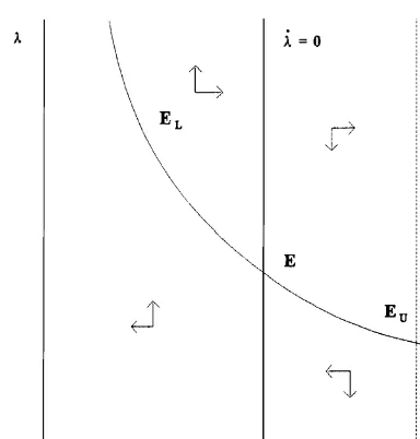
It can be readily veri"ed that the transversality condition (7) is met at the equilibrium point. As shown in Appendix A, the equilibrium dynamics depend on the sign of the trace of the Jacobian coe$cient matrix of the system. If the trace is negative (positive), called Case A (B) below, the equilibrium is a sink (source). The borderline case of a zero trace remains important in this model, suggesting that the solution curve of the dynamical system, Eqs. (6b) and (8), is a Jordan curve, i.e., a closed curve that does not intersect itself. We discuss these global dynamical features of the system case by case.
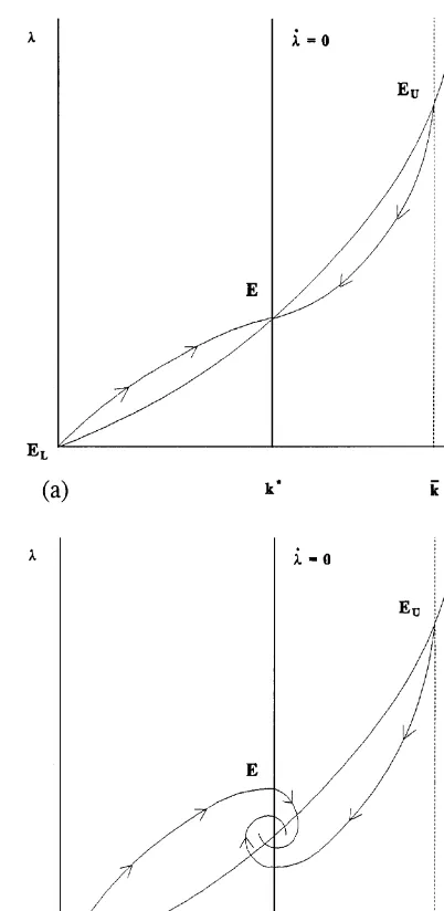
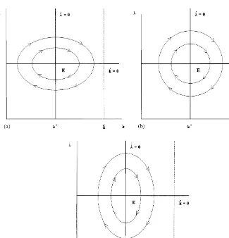
Case A: g '1!p. This case entails the elasticity parameter of utility to government spending,g, to be su$ciently large. First consider the behavior of the trajectories in the phase diagram. The curve for whichjQ"0 is vertical, while the curve for which kQ"0 is upward sloping, which is determined by the following equation:
the phase portraits for the"rst two possibilities, while the transparent borderline case is not drawn. Notably, thejQ"0 locus is the standard modi"ed golden rule for capital accumulation in the presence of taxation and public goods, which says that ultimately the (after-tax) productivity of capital is determined by the rate of time preference. The unique interior equilibrium point is denoted as E. The two loci divide each phase portrait into four regions, where the components of directions of movement are indicated by arrows:jQ'0 in the left-hand side of the locusjQ"0 andjQ(0 in the right; above the locus ofkQ"0,kQ'0, andkQ(0 below it.
Next, this case features that the determinant is positive while the trace is negative. A negative trace and a positive determinant mean that there is a locally indeterminate steady state, i.e., there exists an indeterminate steady state with a continuum of equilibrium trajectories converging to the steady state. In addition, because of the local indeterminacy, there may be stationary sunspot equilibria in the neighborhood of E.
The following proposition presents the results for Case A (see Appendix A):
Fig. 1. The dynamical system for Case A: (a)a[g!(1!p)]'1!b; and (b)a[g!(1!p)](1!b.
E, if g '1!p. More speci,cally, when g
H(g(1, E is a stable node; when
g(g
H,E is a stable focus.
Fig. 2a and b displays these possible kinds of equilibrium dynamics. The two terminal points, at whichk"0 andk"kM, are denoted as E
Fig. 2. The equilibrium dynamic paths for Case A: (a)g
H(g(1; and (b)g(gH.
Fig. 3. The dynamical system for Case B.
analysis makes evident that their subsequent growth experience could dramati-cally di!er, which may be the result of indeterminacy of equilibria, that is, di!erent counties follow di!erent equilibrium trajectories toward a stationary state or a balanced growth path. This result is reminiscent of the recent literature of indeterminacy without public goods, e.g., Benhabib and Farmer (1994) and Benhabib and Perli (1994).
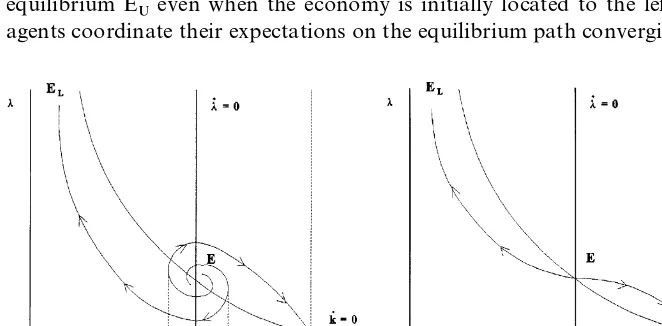
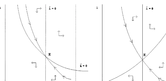
Case B:g(1!p. This case is profoundly di!erent from Case A. First, as shown in Fig. 3, the kQ"0 locus becomes downward sloping and convex (also see Eq. (10)). Second, the local stability of the unique interior equilib-rium E changes drastically: it becomes a source since the trace is positive (see Eq. (A.3) in Appendix A). Third, the lower terminal point, E
L, becomes instead (0,#R), which is equivalent to c"0 via Eqs. (6a) and (10). This state with zero consumption and capital stock can be viewed as a state of poverty and stagnation, which generically corresponds to the &poverty trap' in the literature.
Given that the unique interior stationary point is a source, the solution to the dynamical system will hit either boundary eventually, for any initial values, k0andj0, that satisfyk03(0,kM ). Following Krugman (1991), these two positions
Fig. 4. The equilibrium dynamical paths for Case B: (a)g
L(g(1!p; and (b)g(gL.
impinge on the nature of the characteristic roots for E. As shown in Appendix A, we can state:
Proposition2.Suppose that the following conditions hold:a#b'1,b(1,and
g(1!p.¹hen the unique interior equilibrium E of the system is a source.Ifg
L
(g(1!p, E is an unstable focus;wheng(g
L,E is an unstable node. Wheng
L(g(1!p, the linearized system diverges from the stationary state in expanding oscillations. The kind of equilibrium dynamics is delineated in Fig. 4a, in which perfect foresight paths consist of a pair of interwining, non-crossing spirals around E. As the"gure makes clear, the set of equilibria depends on the size of the initial capital stock relative to the benchmarks k1 and k2, de"ned by the projections onto thekaxis of the left-most point of E
L's stable manifold and the right most point of E
U's stable manifold, respectively. The interval (k
1,k2) is generically called the&overlap'region of the stable manifolds associated with E
Land EU, where the extent of the overlap region depends in a complicated way on parameter values. When initial capital stock falls out of that region, determinate equilibrium dynamics emerge. Ifk
03(0,k1), there exists an equilibrium path that the economy will be trapped in the lower terminal equilibriumE
L. Similarly, if initial level is su$ciently high such thatk0'k2, the economy converges monotonically to E
U. In both circumstances, history dictates the choice of equilibrium in the long run.
Ifk
03(k1,k2), there are multiple trajectories that satisfy all the equilibrium conditions, and the initial condition is no longer su$cient to determine the outcome of the economy in the future. The economy can reach the high equilibrium EUeven when the economy is initially located to the left of E, if agents coordinate their expectations on the equilibrium path converging to E
Given the perfect foresight nature of the model, expectations are entirely self-ful"lling. In addition, the model reveals that starting from the right of E does not guarantee the convergence to E
U. In a word, expectations will matter when the initial capital falls into the overlap region. The policy implication is obvious like that proposed in other studies: to break the vicious cycle of poverty, it calls for active state intervention.
The above result accords reasonably well with intuition. In this model, if
b(1, the level of public services is an increasing function of the level of private
capital, as seen from Eq. (4). Suppose some agents increase their levels of capital. Then the level of public services will increase, which in turn will raise the marginal return of capital and induce everyone to increase capital accumulation. In other words, there gives rise to a positive capital spillover. As argued by Krugman (1991) and Matsuyama (1991), if expectations are coordinated in a way that everyone believes that the economy will end up in the high equilib-rium, then it will.
Wheng(g
L, E possesses two distinct, real, positive eigenvalues. Hence, the only compatible portrait belongs to a scenario that determinate perfect foresight paths emerge in that the linearized system steadily diverges from the stationary state, no matter where the economy starts. Fig. 4b depicts this case. There is a &threshold' for capital: whenk
0 ( k*, the economy converges to the low terminal point E
L; whenk0'k*, it converges to the high terminal point EU. Clearly, history plays a decisive role in determining the long-run position of the economy.
¹he borderline case:g"1!p. Denote this value asg
0. This case remains the most interesting one, because economic cycles now take place. To show this, we notice that the determinant is positive, while the trace is equal to zero, thereby implying that the Jacobian has a pair of pure imaginary eigenvalues. If we de"ne a real positive number tively. Moreover, it is straightforward to show that at g"g
0, the real part of the derivative of eigenvalue with respect to g does not vanish. Thus, the loss of stability can be guaranteed by small perturbations in the bifurcation parameter g. According to the Hopf bifurcation theorem (Guchenheimer and Holmes, 1990), it follows that
Proposition3.Suppose thata#b'1,b(1,andg"1!p.¹hen,there exist economic cycles}the Hopf bifurcation}in the system.
8From the initial and subsequent positions, we can see that the points move clockwise. write the Jacobian of the system, evaluated at g"g
0, as (also see Eq. (A.1) in These equations can be transformed into a standard second-order equation for x(g
0): d2x(g
0)
dt2 #J12(g0)J21(g0)x(g0)"0. (13) Similarly, one can obtain the same equation fory(g
0). Eq. (13) is the well-known van der Polequation in the absence of damping. In order to determine a particu-lar solution, we now need two side conditions on the path of each variable. Suppose that the system initially starts at the point (0,y
0). The other condition for each variable is then determined by Eqs. (12a) and (12b). Accordingly, the system settles into the following oscillations:
y
0). It is observed that the amplitude of thextoscillation, y
0[J21(g0)/J12(g)0)]1@2, plays a crucial role in shaping the cycles. Attention now turns to determine the relative magnitude ofJ
the equilibrium ratio ofjH(g
Fig. 5a}c depicts the three possibilities, in which thekQ"0 locus is horizontal.
Next, the stability conditions are examined. To make the attempted task manageable, we still work with the linearized system but slightly perturb the bifurcation parameterg, while all other parameters remain"xed. The resulting Jacobian as opposed to Eq. (11) is
J,
C
0 positive, while that of J22 is indeterminate. Wheng approaches g0 from the above (below), J22 is negative (positive). The presence of this term yields the following equations:
yR"!J
12x, (16a)
xR"J
21y#J22x. (16b)
Consequently, we can obtain the more general version of the van der Pol equation
12J21)1@2. J22 is the so-called damping rate. It is known that a positive (negative) value forJ
22means that the amplitude of the oscillations grows (decays); also see Appendix B. Thus, we can prove the following result:
Proposition5.¹he stability of the bifurcated cycle is determined by the sign of J 22. If J
Fig. 5. The equilibrium dynamic paths for the Borderline Case: (a) J
21(g0)'J12(g0); (b)
J
21(g0)"J12(g0); and (c) J21(g0)(J12(g0).
9It can be shown that the case of decreasing returns to scale produces qualitatively the same implication, except that Cases A and B are simply switched.
It should be pointed out that estimates of the preference parameterspandgin a framework with utility-enhancing public services have not yet been obtained. As a result, the question of whether there are economic cycles in the borderline case ofg"1!premains unanswered. At this stage, we are still unable to rule out such a possibility. Hopefully, our theoretical demonstration of the potential importance of this case may encourage empirical work on this issue.
4. The case of strong increasing returns to scale
In this section, we brie#y consider a special case of increasing returns: the share of public services in production,b, exceeds one, i.e.,b'1.9Unlike what happened in the previous section, the local stability of the unique stationary state E and the entire equilibrium dynamics completely change. First, the shapes of the kQ"0 locus alter for both Cases A and B. From Eq. (11), the curve becomes downward sloping for Case A, while upward sloping for Case B. Moreover, in Case B, the locus can be either convex, or concave, or a straight line from the origin, depending on certain parameter values.
Second, the local stability of E changes as well. The condition ofb'1 (or equivalently c(0) makes the determinant negative (see Eq. (A.2) in Appen-dix A), which yields:
Proposition 6. =hen increasing returns are so strong that b '1, the unique
equilibrium is a saddle point.
This proposition holds because one of the roots of the coe$cient matrix is positive and the other is negative. Fig. 6a and b displays the phase portraits for Cases A and B, and similar diagram can be drawn for the borderline case. These "gures suggest that given an initial capital stock k
03(0,kM ), there is a unique equilibrium path, which converges monotonically to the stationary state. That path belongs to the stable manifold of the stationary state.
Fig. 6. The equilibrium dynamic paths forb'1: (a) Case A; and (b) Case B.
5. Concluding remarks
In this paper we have examined the implications of relaxing the standard assumption}the production function exhibits socially constant returns to scale }in a simple growth model with public goods. It was found that the model is capable of generating a whole spectrum of interesting dynamics, which do not arise with constant returns. Two features are worth noting for the case of moderate increasing returns. The "rst one involves in a possibility that the dynamic path diverges from an interior equilibrium in expanding oscillations, suggesting that self-ful"lling expectations play an essential role in determining the long-run position of the economy. The second one is that economic cycles take place, implying that the endogenously determined government spending is also periodic when the system is in the neighborhood of the equilibrium.
Our"ndings are obtained within a decentralized stationary framework. We believe, however, that the model can be extended to more general settings, such as incorporating public investment and endogenizing government deci-sions. Another interesting extension lies in allowing the government budget to be balanced in a present value sense and analyzing the implication of this modi"cation.
Acknowledgements
10gHis obtained directly from Eq. (A.4) by setting the right hand side to zero and noting that
g'1!p. To yield meaningful discussion, we require thatg
H(1, which is generally warranted
under a wide range of parameter values, e.g., the scale parameterbis in the left neighborhood of one.
Appendix A. Dynamic analysis
Linearizing Eqs. (6b) and (8) in the vicinity of the equilibrium de"ned in Eq. (9) yields
The determinant and the trace of this Jacobian can be computed as
Det"o2(a#b!1)
ac '0, (A.2)
Trace"o[(1!p)!g]
c , (A.3)
where use has been made ofc(,(1!b)(1!p))'0. Since the determinant of the Jacobian of Eq. (A.1) measures the product of the roots and the trace measures the sum, one can use information on the sign of determinant and trace to check the dimension of the stable manifold of the steady state. From Eq. (A.2) and (A.3), we can only determine the sign of the determinant, which is positive, implying that the two characteristic eigenvalues of the linearized system are of the same sign. In other words, a positive determinant can be associated with either a stable manifold of dimension zero (an unstable steady state) or a stable manifold of dimension two (a completely stable steady state), depending on the sign of the trace. Given that the sign of the trace is indeterminate, we can distinguish among the following two cases (the borderline case is discussed in detail in the text and in Appendix B):
Case A:g'1!p. The trace is negative, suggesting that the equilibrium is a sink. That is, the corresponding steady state is locally indeterminate.
The discriminant of the coe$cient matrix in Eq. (A.1) is
D"(Trace)2!4 Det"o2
By"xing all parameters except forgin Eq. (A.4), we"nd that there exists a value ofg, denoted bygH:10
g
such that (1) ifg
H(g(1, the system has two distinct, real, negative roots. The steady state is a stable node; and
(2) ifg(g
H, the eigenvalues form a complex conjugate pair with a negative real part. The steady state is a stable focus.
Case B:g(1!p. The trace is positive, suggesting that the equilibrium is a source. There exists a value ofg, denoted byg
L:
g
L"(1!p)!2Jc(a#b!1)/a, (A.6) such that the stability properties change whengcrosses this value. The following generic con"gurations are possible:
(1) when g
L(g(1!p, the system has a pair of imaginary roots with positive real parts. The steady state is an unstable focus; and
(2) wheng(g
L, the system possesses two distinct, real, positive eigenvalues. The steady state is an unstable node.
Appendix B. Proof of Proposition 5
The procedure we shall use is called&the method of slowly varying amplitude and phase' (see, e.g., Sanders and Verhaulst, 1984). Inspection of Eq. (17) indicates that if the right-hand side were zero, then x would oscillate sinusoidally in time [see Eq. (14b)]. This leads us to introduce the following expressions forx and its time derivative [see Eq. (12b)]:
x
t"atsin(ut#/t), (B.1) xR"a
tucos(ut#/t), (B.2)
wherea
5and/5are time-varying amplitude and phase, respectively. Notice that Eq. (B.2) is not the usual derivative ofx
t, which in fact is equal to
xR"aR sin(ut#/)#a(u#/Q) cos(ut#/). (B.3)
Equating Eq. (B.3) with (B.2), it produces
aR sin(ut#/)#a/Q cos(ut#/)"0. (B.4) The second derivative ofxcan be computed from Eq. (B.2):
x("aRucos(ut#/)!au(u#/Q)sin(ut#/). (B.5)
Substituting Eqs. (B.5) and (B.2) into Eq. (17) and rearranging yield
aR cos(ut#/)!a/Q sin(ut#/)"J
Next, we derive two equations for aR and /Q. Using the following algebraic
It should be noted that Eqs. (B.7) and (B.8) are equivalent to Eq. (17). Now, we invoke the crucial idea of the method of slowly varying amplitude and phase: when a trajectory gets closer to the limit cycle, its amplitudeaand phase/vary slowly over the time scale of the period of oscillation. Therefore, the time derivatives of these variables are roughly constant over one period of oscillation. On the basis, we integrate the right-hand sides of Eqs. (B.7) and (B.8) over one period and treat the amplitude and phase in these integrations as constants. Making use of the following integrals:
u
22"0, the limit cycle is reached. To "nd the rate at which a nearby trajectory approaches the cycle, Eq. (B.9) alludes that it invokes an exponential relation, which depends on the sign ofJ
22. IfJ22'(() 0, the amplitude of oscillations,a
t, grows (decays).
References
Abe, N., 1995. Poverty trap and growth with public goods. Economics Letters 47, 361}366. Barro, R., 1990. Government spending in a simple model of endogenous growth. Journal of Political
Economy 98, S103}S125.
Barro, R., Sala-i-Martin, X., 1992. Public "nance in models of economic growth. Review of Economic Studies 59, 645}661.
Benhabib, J., Farmer, R., 1994. Indeterminacy and increasing returns. Journal of Economic Theory 63, 19}41.
Benhabib, J., Perli, R., 1994. Uniqueness and indeterminacy: on the dynamics of endogenous growth. Journal of Economic Theory 63, 113}142.
Glomm, G., Ravikumar, B., 1994. Public investment in infrastructure in a simple growth model. Journal of Economic Dynamics and Control 18, 1173}1187.
Guchenheimer, J., Holmes, P., 1990. Nonlinear Oscillations, Dynamical Systems and Bifurcations of Vector Fields. 3rd ed., Springer, New York.
Krugman, P., 1991. History versus expectations, Quarterly Journal of Economics 106, 651}667. Matsuyama, K., 1991. Increasing returns, industrialization, and indeterminacy of equilibrium.
Quarterly Journal of Economics 106, 617}650.
Sanders, J., Verhaulst, F., 1984. Averaging Methods in Nonlinear Dynamical Systems. Springer, New York.
![Fig. 1. The dynamical system for Case A: (a) �[�!(1!�)]'1!�; and (b) �[�!(1!�)](1!�](https://thumb-ap.123doks.com/thumbv2/123dok/3104534.1376540/7.468.91.307.51.469/fig-dynamical-case-b.webp)