USING MULTI-DIMENSIONAL MICROWAVE REMOTE SENSING INFORMATION
FOR THE RETRIEVAL OF SOIL SURFACE ROUGHNESS
P. Marzahn a*, R. Ludwig a
aDepartment of Geography, Ludwig-Maximilians-University Munich, Germany – [email protected]
KEY WORDS: Radar, SAR, PolSAR, Soil Surface Roughness, airborne, in-field measurements
ABSTRACT:
In this Paper the potential of multi parametric polarimetric SAR (PolSAR) data for soil surface roughness estimation is investigated and its potential for hydrological modeling is evaluated. The study utilizes microwave backscatter collected from the Demmin test-site in the North-East Germany during AgriSAR 2006 campaign using fully polarimetric L-Band airborne SAR data. For ground truthing extensive soil surface roughness in addition to various other soil physical properties measurements were carried out using photogrammetric image matching techniques. The correlation between ground truth roughness indices and three well established polarimetric roughness estimators showed only good results for Re[ρRRLL] and the RMS Height s. Results in form of multi-temporal roughness maps showed only satisfying results due to the fact that the presence and development of particular plants affected the derivation. However roughness derivation for bare soil surfaces showed promising results.
1. INTRODUCTION
As the boundary layer between the atmosphere and the pedosphere the random roughness of natural surfaces, defined as the height deviations from a plain reference in the scale of 2-200mm (Roemkens and Wang, 1986) , plays an important role in numerous physical processes. Several investigations showed the impact of soil micro relief on processes such as wind and water induced soil erosion or the retrieval of near-surface soil moisture as well as their description in respective models (Fohrer et al. 1999). The nature of rough surfaces can be described statistically by means of various roughness indices, like the rms-height, the surface correlation length or the tortuosity index (Taconet and Ciarletti, 2006). Temporal roughness variability is caused by wind or water erosion, agricultural practice or soil sealing and crusting by precipitation or irrigation. However, soil surface roughness is yet only quantitative direct measurable on plots from 0.2 m² up to 20 m², on watershed scale there is no known possibility for direct measurements (Rieke-Zapp and Nearing, 2005, Warner, 1995, Helming, 1995). Thus, roughness is often assumed constant in respective soil infiltration and run-off modeling efforts, introducing strong simplification and considerable data uncertainty (Burt, 1998, Cerdan et al. 2001, Boardman and Favis-Mortlock, 1998). To bridge this scientific gap, the capacity to retrieve this information from multitemporal airborne PolSAR data is investigated.
The presented study is performed in the frame of the ESA-funded project AgriSAR 2006 started April 19th and ended in July 26th. A major component of this study was to generate an image and ground data base for the examination and validation of bio-/geo-physical parameter retrievals, obtained at different radar frequencies and polarisations (X-, C- and L-Band) from the airborne sensor E-SAR, operated by the German Aerospace Center (DLR). E-SAR flights were performed during the whole agri-phenological cycle in the well consolidated test-site of Demmin, Mecklenburg Western-Pomerania, in the North-East of Germany.
* Corresponding author
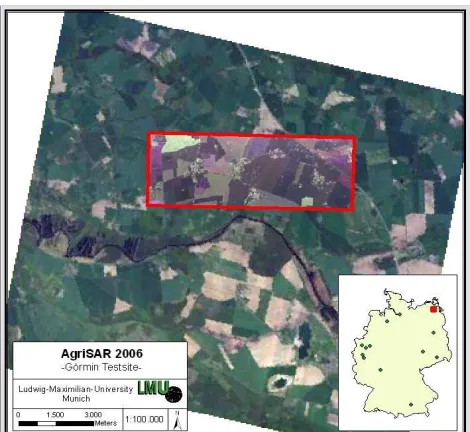
Figure 1. Overview of DEMMIN-Görmin Testsite in the North East of Germany
2. METHODS
2.1 Test-Site
2.2 In-field Measurements
Roughness measurements were performed using photogrammetric imaging techniques. For roughness survey a portable tripod was developed were a calibrated Rollei d7 metric digital camera and 12 high accurate (3/10 mm) ground control points (GCP) were fitted. Images were taken from approx. 118 cm height above ground and the height-base ratio was approx. 2.5. The horizontal coverage of the stereomodel is 70x70 cm².To get information on soil surface roughness of vegetated sample points the vegetation was carefully cut off direct above the ground and removed from the scene.
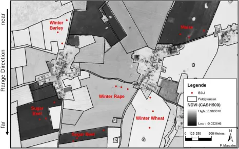
Figure 2. location of sample points (red). (101: Winterrape; 222: Maize; 250: Winterwheat; 440: Winterbarley;
102+460: Sugarbeet).
The three dimensional surface reconstruction was done by using Leica Photogrammetry Suite LPS software.Exterior orientation of the two images was established using bundle block adjustment techniques. Therefor, additionally to the 12 known GCPs, tie-points were derived and their three dimensional coordinates were calculated by bundle block adjustment. Best results in bundle block adjustment were achieved by using a additional 12 parameter model (Ebner Model). The achieved accuracy from the exterior orientation is in z=0.8 mm and in xy=0.37 mm refered to the known GCPs.
For derivation of the DSMs different strategies had been developed. Thus, LPS works in epipolar lines the strategies vary only in the x-direction depending on the degree of soil sealing. Minimum correlation coefficient was set to 0.65.
2.3 Roughness Characterization
To quantify the soil surface roughness the rms-height s had been calculated from the derived DSMs. The rms-height is definded as the standard deviation of the heigth values Z:
(1)
(2)
where k is the wave number and λ is the wavelength in cm.
2.4 Ancillary Field Measurements
To quantify a potential impact from the vegetation and/ or soil on the radar backscatter, several vegetation and soil parameters
had been acquired in addition during each campaign at the sample points shown in Fig. 2. To derive soil moisture, soil samples were taken in 0-5 cm and 5-10cm by 100 cm³ Kopecky Rings. The soil samples were dried out in an oven and volumetric soil moisture was calculated. In addition, vegetation height, Leaf-Area-Index (LAI) crop coverage, and biomass (wet/dry) had been measured in the fields.
Furthermore an agro-meteorological station recorded precipitation, air- and soil temperature, wind direction, -speed, short wave and long wave radiation every 10 minutes.
2.5 Radar Data
A total of 11 respective E-SAR flights recorded radar data during the summer agri-phenological cycle in 2006. Delivered data products were X- (single pol.), C- (dual) and L-Band (quad) data in radar geometry images (RGI) and geocoded and terrain corrected products (GTC).
For data analysis geocoded SLC L-Band Data was chosen to derive the roughness information. As shown by Thiel et al. (2001) it is feasible to use geocoded SLC L-Band data to perform decomposition algorithms.
The radar data was speckle filtered by applying a 7x7 window enhanced LEE-Filter.
To obtain an improved understanding of the involved scattering mechanisms, a Cloude decomposition of the backscatter signal was performed using a 5x5 box-car filter. It distinguishes the dominant scattering process (surface, volume or double-bounce) by means of the alpha angle and allows to determine the proportional fraction of the other scattering components in terms of backscatter entropy and anisotropy.
For roughness determination, three well established roughness estimators were calculated: surface roughness on bare soil fields. Cloude (1999) and Cloude and Lewis (2000) introduced two inverting approaches depending on roughness states to estimate soil surface roughness. Note that the autocorrelation length is unconsidered for estimation.
2.5.2 Circular polarization Coherence
The circular coherence is defined as:
2 electric field vector about the line of sight. Mattia et al. (1997) verified first a significant sensitivity of the circular coherence due to surface roughness while the impact of the dielectric constant is reduced. As roughness increases the circular coherence decreases.
2.5.3 Real part of the circular polarization coherence
The real part of the circular coherence was first introduced by Schuler et al. (2002) and is defined as:
2
It is a further development of the circular coherence with the advantage of not using the imaginary part of the circular coherence which is sensitive to unsymmetrical scattering contributions such as vegetation. Furthermore it is very insensitive to parameters such as the dielectric constant. However, for an azimuthal symmetric surface both estimators are the same, in particular, |ρRRLL| becomes real and therefore equals Re[RRLL]. Same holds for A.
The real part of the circular coherence was calculated by applying a 5x5 window box-car filter.
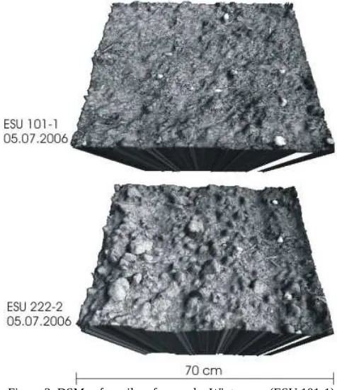
Figure 3. DSMs of a soil surface under Winterrape (ESU 101-1) and under Maize (222-2) after receiving 87 mm
precipitation since monitoring.
3. RESULTS
3.1 Field Data
A total of 176 micro DSMs were derived using photogrammetric techniques over the whole agri-phenological cycle. The derived DSMs showed good agreement with high accurate, manually measured reference points with a mean absolute error of 1.2mm and RMSE of 1.6mm. Fig. 3 shows two example DSMs. ESU 101-1 indicates a soil surface under Winterrape, ESU 222-2 under Maize. Both received approx. 87 mm precipitation since monitoring. As can been seen in Fig 3, it
is possible to distinguish between different aggregates and even small aggregates can be detected. For quantitative analysis, roughness indices were calculated as specified in 3. Table 1 summarizes the statistical properties of the obtained rms-heights.
Roughness indices indicated rough surfaces for all sample points after calculating the Fraunhofer criterion.
Field 101
s_mean 0.8 0.9 0.91 1.07 1.74 1.29
s_max 1.2 1.2 1.2 1.8 2.9 2.4
s_min 0.6 0.7 0.8 0.8 1 0.9
Table 1. Statistical values of in-field ks values .
Figure 4. Examples of calculated roughness estimators from fully polarimetric L-Band data acquired at the 19th
of April 2006
3.2 Radar Data
According to equations 3-5 the potential roughness estimators were calculated from the E-SAR data. As an example, Fig. 4 shows the spatial distribution of the different roughness estimators. It can be observed, that the different estimators represent the roughness conditions on the agricultural fields. However, with different sensitivities and values.
Table 2, the correlation showed only poor results between the potential roughness estimators and ks. Except Re[RRLL] which showed a fairly good dependency from ks. Note, that these results were retrieved from calculating correlation coefficients for all the data and by not separating different scattering mechanisms in the calculation.
Parameter R² r m
A 0.00 0.03 0.03
|ρRRLL| 0.02 -0.16 -0.08
Re[ρRRLL] 0.11 0.32 0.13
Table 2. Correlation parameters between roughness estimator and ks values for all data points.
To exclude a potential influence or bias of the signal from other variables (soil moisture, biomass, crop cover), a correlation test was carried out. However , no significant correlation could be retrieved, either for soil moisture nor vegetation parameters (data not shown).
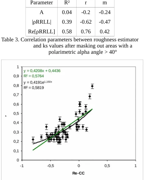
As there was no significant correlation between the afore mentioned additional variable and the potential roughness estimator, an additional test was carried out including the dependency of the correlation coefficients per day from the scattering mechanisms . Therefore the polarimetric alpha angle was calculated and plotted against the correlation coefficients. Fig. 5 shows the output of this analysis. As can be seen, for most of the potential roughness estimators, the correlation coefficients change their signs at a polarimetric alpha angle of ~40°. Therefore, we chose this as a threshold to mask out non valid areas. Table 3 shows the regression parameters of the potential roughness estimators and ks for areas with a polarimetric alpha angle below <40°. As can be seen, the real part of the circular coherence outperforms the magnitude of the circular coherence as well as the anisotropy. There is also an increase in the amplitude of the correlation coefficients compared to Table 2.
Figure 5. Correlation coefficients between roughness estimators and ks versus mean polarimetric alpha angle showing threshold for valid areas of roughness
retrieval.
Parameter R² r m
A 0.04 -0.2 -0.24
|ρRRLL| 0.39 -0.62 -0.47
Re[ρRRLL] 0.58 0.76 0.42
Table 3. Correlation parameters between roughness estimator and ks values after masking out areas with a
polarimetric alpha angle > 40°
Figure 6. Correlation (linear black line, exponential green line) between ks [cm] and Re[RRLL] (Values ks<0.27
cm (~ s = 1cm) are masked out).
The correlation between ks and Re[RRLL] is shown in Fig. 6 as a scatter plot. Besides using a linear regression model, an exponential model would lead to a slightly stronger relationship.
Based on the correlation between s and Re[RRLL] the surface roughness for the whole investigation area was estimated. Fig. 8 shows as an example the estimated soil surface roughness based on the correlation. Invalid areas with a polarimetric alpha angle > 40° as well as settlements, forest and streets are masked out in black. Note, that the showed roughness values are real rms-heights and not scaled with the wavenumber of the applied L-Band SAR data (eg. s not ks).
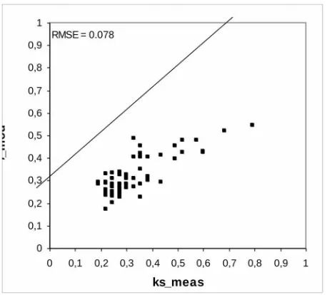
Figure 7. Modeled versus measured ks values
Figure 8. Spatial distribution of s . Invalid areas with polarimetric alpha angle α > 40° are masked out
black
3.3 Multi-temporal roughness analysis
For each campaign day, roughness maps were calculated based on the correlation shown in Fig. 6. The developing of the roughness states for the whole agri-penological cycle is shown in Fig. 9 and Fig. 10.
It is obvious in both figures that the roughness state is changing over time. Under winter vegetation (Fig. 9) such as Winterrape
Figure 9. Roughness developing for the sample points 101 (WR), 250 (WW) and 440 (WB).
Figure 10. Roughness developing for the sample points 102 (SB), 222 (M) and 460 (SB)
(101) the roughness decreases slightly. For Winterwheat and Winterbarley a stronger decrease of roughness can be observed until the 17th of may. Than Winterwheat stays quite low (s= 1.2-1.4 cm) while the roughness state of the Winterbarley field increases slightly again. This causes the suspicion that the roughness estimation for the Winterbarley field is influenced by vegetation, indeed statistical analyses showed no impact. In general it is to note, that the soil surface roughness under winter resistant vegetation is overestimated by means of 0.8 cm without any impact from vegetation
The developing of roughness states for soil surface under summer vegetation (102, 460 (SB), 222 (M)) shown in Fig. 10 is similar to the winter vegetation (Fig. 9). For the Maize field (222) a decrease can be observed. Indeed the roughness measured values for s in the field are 0.2 cm higher than the estimated roughness values. Both of the Sugarbeet fields show first a strong decrease in soil surface roughness until the 7th of june and then show a continuous increase very similar to the groth of the Sugarbeet plants. However, a multiple regression between the roughness values, vegetation parameters and Re[RRLL] showed only a strong relationship between the values on field 460. On field 102 there was no relationship measurable. For the Sugarbeet fields an overestimation of roughness can be observed in average of 0.21 cm for the field 102 and 0.26 cm for 460.
4. CONCLUSIONS
As shown in this investigation, only the real part of the circular polarization coherence is sufficient correlated with the rms-height measured under natural conditions over a wide range of soil surface roughness states, outperforming any other potential correlation or roughness index. These results verify the investigations by Schuler et al (2002) and Thiel (2003). However, this investigation shows, that Re[RRLL] is not only sensitive to soil surface roughness. Even tough an influence on Re[RRLL] from vegetation could not be quantified with the obtained standard vegetation parameters it is obvious that the developing of plants affect the estimation of s through Re[RRLL]. This assumption is also supported by the dependency of the retrieved correlation coefficients from the polarimetric alpha angle, which allow only an estimation of soil surface roughness from PolSAR data for areas with dominant surface scattering. Finally the proposed method allows for an accurate retrieval of soil surface roughness with an RMSE of 0.1 cm compared to infield measurements.
REFERENCES
BURT, T.P., “Infiltration for soil erosion models: some temporal and spatial applications”. In: Modelling soil erosion by water. NATO-Series I-55, ed. BOARDMAN, J., D.T. FAVIS MORTLOCK pp. 213-224. Berlin 1998
CERDAN, O., V. SOUCHÈRE, V. LECOMTE, A. COUTURIER and Y. LE BISSONNAIS, “Incorporating soil surface crusting processes in an expert-based runoff model: Sealing and Transfer by Runoff and Erosion related to Agricultural Management – STREAM”. Catena
Vol. 46, pp 189-205, 2001
CLOUDE, S. R., “Eigenvalue parameters for surface roughness studies”. Proceedings of SPIE Conference on Polarisation: Measurement, analysis and remote Sensing II. Denver Colorado, 1999
CLOUDE , S. R. and G.D. LEWIS, “Eigenvalue analysis of Mueller Matrix for bead basted aluminium surfaces” Proceedings of SPIE Conference on Polarisation analysis and measurement III, 2000 FOHRER, N., J. BERKENHAGEN, J.-M. HECKER and A,
RUDOLPH, “Changing soil and surface conditions during rainfall single rainstorms/ subsequent rainstorms”. Catena Vol. 37, pp. 355-375, 1999
HAJNSEK, I. “Inversion of surface parameters using Polarimetric SAR”. Jena, 2001
HELMING, K., „Die Bedeutung des Mikroreliefs für die Regentropfenerosion“. Bodenökologie und Bodengenese Nr. 7, Berlin 1992
HELMING, K., CH. H. ROTH, R. WOLF and H. DIESTEL, “Characterisations of rainfall – mircrorelief interactions with runoff using parameters derived from digital elevation models (DEMs)”.
Catena Vol. 6, pp. 273-286, 1993
MATTIA, F., T. LE TOAN, J.C. SOUYRIS, G. DE CAROLIS, N. FLOURY, F. POSA and G. PASQUARIELLO, “The effect of surface roughness on multi- frequenzy polarimetric SAR data”.
IEEE Trans. Geosci. Remote Sensing, Vol 35 954-966, 1997 RIEKE-ZAPP, D. and M. A. NEARING, “Digital close range
photogrammetry for measuremnet of Soil erosion”. The Photogrammetric Record, Vol 20, 69-87, 2005
ROEMKENS, M.J. and J.Y. WANG, “Effect of tillage on surface roughness”. Trans. ASAE Vol 29, pp 429-433, 1986
SCHULER, D. L., J.S. LEE and D. KASILINGAM, “Surface roughness and slope measurements using polarimetric SAR data”. IEEE Trans. Geosci. Remote Sensing, Vol 40, 687-698, 2002
TACONET, O. and V. CIARLETTI, “Estimating soil roughness indices on a ridge-and-furrow surface using stereo photogrammetry”. Soil Till. Res. In Press 2006
THIEL, CH, “Measuring surface roughness on base of the circular polarization coherence as an input for simple inversion of the IEM model”. Proceedings of PolInSAR Workshop, 14.-16.01.2003, Frascati, Italy, 2003
THIEL, CH., S. GRUENLER, M. HEROLD, V. HOCHSCHILD, G. JAEGER and M. HELLMANN, „Interpretation and Analysis of Polarimetric L-Band E-SAR-Data for the Derivation of Hydrologic Land Surface Parameters”. IEEE Proceedings IGARSS’01, Sydney 2001