FIXED-WING MICRO AERIAL VEHICLE FOR ACCURATE CORRIDOR MAPPING
M. Rehak, J. Skaloud
École Polytechnique Fédérale de Lausanne (EPFL), Switzerland - (martin.rehak, jan.skaloud)@epfl.ch
KEY WORDS: corridor mapping, MAV, UAV, GNSS/INS, boresight, calibration
ABSTRACT:
In this study we present a Micro Aerial Vehicle (MAV) equipped with precise position and attitude sensors that together with a pre-calibrated camera enables accurate corridor mapping. The design of the platform is based on widely available model components to which we integrate an open-source autopilot, customized mass-market camera and navigation sensors. We adapt the concepts of system calibration from larger mapping platforms to MAV and evaluate them practically for their achievable accuracy. We present case studies for accurate mapping without ground control points: first for a block configuration, later for a narrow corridor. We evaluate the mapping accuracy with respect to checkpoints and digital terrain model. We show that while it is possible to achieve pixel (3-5 cm) mapping accuracy in both cases, precise aerial position control is sufficient for block configuration, the precise position and attitude control is required for corridor mapping.
1. INTRODUCTION
Unmanned Aerial Vehicles (UAV) are nowadays a well-established tool for mapping purposes. They represent an achievable technology for various geomatic tasks including photogrammetry. Their popularity comes from the effectiveness and operational costs (Colomina and Molina, 2014). One of the mapping fields with high potential for UAVs is corridor mapping. Such mapping is important for highway planning, environmental impact assessment, infrastructure asset management as well as for power line and utility pipeline surveys.
Corridor mapping is challenging in several aspects. If we neglect the issue of safety, maintaining good geometry and assuring demanded accuracy of the final mapping products are the main difficulties. The latter depend on the number and distribution of ground control points and/or accuracy of directly measured exterior orientations (EO) of imaging data. Indeed, corridor mapping is a type of photogrammetric imagery where the images are taken in series of continuously overlapping photos. The latter constitutes of either just one or more strips, however, not representing a typical block structure. But it is only the latter method that provides an effective compromise between the coverage and amount of data collected during a mission.
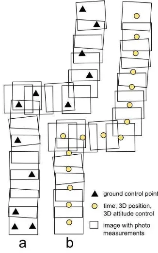
Such a configuration is schematically depicted in Figure 1 together with requirements on image orientation. Even when considering a favourable image texture that allows automated measurement of a large number of tie-points, the absolute image orientation is in the case of indirect sensor orientation (a) stabilized by a large number of ground control points (GCP), while in the case of integrated sensor orientation (b) by the on-board observations of EO.
In other words, in the absence of precise aerial position and attitude control, the lack of significant lateral overlap in single or double strip operations requires that absolute orientations of images are passed from the ground up. Technically, for today’s MAVs, there are only two ways how to deal with such problem: either establish a sufficient number of GCPs along and on both sides of the corridor or perform a block-structure flying path. Despite the obvious difficulties, several rather long corridor
mapping projects have been presented using indirect sensor orientation approach (Delair-Tech, 2014; senseFly, 2015). These data collection activities require time- and labour-intensive efforts which may be difficult to realize in corridors surrounded by high vegetation. Further orientation problems occur when flying over terrain of uniform or instable texture, e.g. snow or coastal areas.
Figure 1. A schematic sketch of corridor mapping configurations
1.1 Problem Formulation
Image orientation is a key element in any photogrammetric project since the determination of three-dimensional coordinates ISPRS Annals of the Photogrammetry, Remote Sensing and Spatial Information Sciences, Volume II-1/W1, 2015
from images requires the image internal and external orientation to be known. In MAV photogrammetry, this task has been exclusively solved using indirect orientation from GCPs and camera self-calibration. There, a sufficient image overlap, a high number of tie-points and a regular distribution of GCPs are the key elements in MAV mapping. By using GNSS measurements as additional observations, the need for GCPs can be eliminated if a geometrically stable block of tie-points can be formed (Heipke et al., 2002; Jacobsen, 2004). On the other hand, when orienting images in a weak block geometry without GCPs, typically in a single strip, we lack precision of attitude determination (Colomina, 1999). Thus, the overall accuracy of the project degrades significantly.
By using an inertial measurement system (INS), the orientation of the images can be determined directly (Schwarz et al., 1993; Colomina, 2007). Therefore, an accurate aerial control via the GNSS/INS system can overcome the need of GCPs in all situations (Colomina, 1999), with practical demonstrations on larger systems several decades ago (Skaloud et al., 1996; Skaloud and Schwarz, 2000; Mostafa, 2002).
Nevertheless, the limited weight, volume and power availability in a MAV payload poses a major challenge when determining accurate orientation on-board. This is especially true for inertial sensors rather than for GNSS receiver/antenna equipment. On the other hand, the requirements on the quality of on-board attitude determination are somewhat relaxed due to the low flying height of a MAV. Due to legal restrictions as well as the optical resolution of carried imaging sensors this is often between 100-250 m above the ground with expected ground sampling distance (GSD) of 3-5 cm. This translates to a permissible noise in attitude determination of 0.01-0.017 deg. For that, lightweight but still performing inertial measurement units (IMU) based on micro-electro-mechanical (MEMS)
technology are good alternatives in terms of weight, power and performance. Nevertheless, a comprehensive state of the art calibration and modelling of sensor errors are essential and so is the mitigation of sensor noise. In this perspective, utilization of several IMUs in parallel, so-called Redundant IMU (R-IMU), is of a great potential (Waegli et al., 2010). It is based on a principle of combining several IMU sensors into one complex system that follows the dynamic of a vehicle with increased reliability and performance (Waegli et al., 2008). In this study we have built a fixed-wing MAV into which we integrated a camera with GNSS/R-IMU sensors. We precisely synchronized and calibrated these sensors and tested their performance on a MAV and during a car test (Rehak et al., 2014).
1.2 Paper Structure
The following part of this article describes the developed fixed-wing MAV platform. We show the potential of integrating a low-cost and off-the-shelf hobby airplane frame with an open-source autopilot, state-of-the-art navigation components and mass-market camera. Then, we concentrate on the problematic of sensor integration and calibration. In particular we focus on determination of positional and angular offsets between imaging and navigation sensors. The last part is devoted to a case study. We first present a self-calibration flight, where we show the accuracy of EO parameters measured on-board. Then we focus our analysis on corridor mapping. The mapping accuracy is evaluated on a calibration field with regularly placed check points. Finally, the last part draws conclusions from the
conducted research work and gives recommendations for further investigations.
2. SYSTEM DESIGN
2.1 MAV Platform
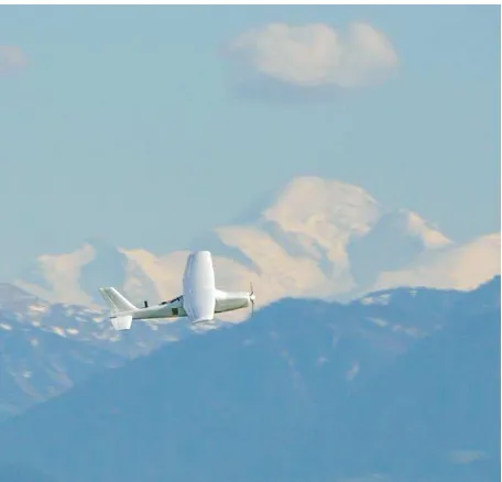
The plane is based on a popular hobby platform (Modellsport GmbH, 2015). The plane is by its form naturally very stable in flight and offers a large internal compartment for the photogrammetric payload. It has a wingspan of 1630 mm and length of 1170 mm. The maximal payload capacity is around 800 g. The operational weight varies between 2200-2800 g, Figure 2. The aircraft is made of expanded polypropylene foam. Despite the weight, the flexible nature of the construction material makes the platform resistant to damage. The plane is easy to assemble and repair with ordinary hobby-grade tools. The cost of the system components is significantly lower with respect to size and endurance comparable platforms (MAVinci, 2015). The endurance with 600 g payload, is approximately 40 minutes. The plane is controlled by Pixhawk autopilot that has been intensively developed over the last few years (Meier et al., 2012). This open-source autopilot unit includes MEMS gyroscopes and accelerometers, 3-axis magnetic sensors, a barometric pressure sensor and an external single frequency low-cost GPS receiver. In our configuration, this receiver has been, however, replaced by a constellation and multi-frequency GNSS board that serves for controlling the autonomous flights as well as for positioning the images (Javad, 2015). The platform takes off from hand and is capable of performing fully autonomous flights. Its mapping missions are programmed within a software called Mission Planner (Ardupilot, 2015).
Figure 2. Fixed-wing platform in flight with Mt. Blanc in background
2.2 Optical Sensor
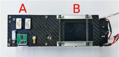
The chosen optical sensor is the off-the-shelf camera Sony NEX 5R. The quality of this mirror-less camera is comparable with SLR (Single-lens reflex) cameras despite being considerably smaller (only 111x59x38 mm) and lighter (210 g for the body). These properties make it highly suitable for UAV platforms. In this particular configuration, the camera is equipped with a 16 mm fixed Sony lens (70 g), which has a reasonable optical quality and offers sufficient stability of the interior parameters (IO) within a mission. The camera is modified for better performance and integration into a MAV system. The camera is triggered electronically and powered from the main on-board power system. The time-stamping of exposures in GPS-time is done via flash synchronization. One of the main constrains for accurate attitude determination is to maintain the orientation stability between a camera and the IMU (Skaloud, 2006). Therefore, the employed R-IMU was rigidly attached to the camera by a custom holder made from carbon as depicted in the Figure 3, which ensures such stability needed for correct sensor orientation. By custom modifications we created and advanced mapping system that can be used on various platforms. The weight of the mount with mapping sensors is 600 g.
Figure 3. Camera sensor head; A – Redundant IMU, B – Sony NEX 5R camera
2.3 GNSS receiver
We employ a geodetic-grade GPS/Glonass/Galileo multi-frequency receiver from Javad with L1/L2 GPS/Glonass antenna (Maxtena, 2014). The receiver has RTK (Real Time Kinematics) capability and 10 Hz sampling frequency. A similar setup is used as a base station for carrier-phase differential processing. Furthermore, the receiver is equipped with a radio modem for RTK corrections.
2.4 Inertial Sensors
In this study we employ the in-house developed FPGA-board (Field-Programmable Gate Arrays) called Gecko4Nav comprising of two MEMS IMUs NavChip (Intersense, 2012), all precisely synchronized to the GPS time-reference (Kluter, 2012). The Gecko4Nav contains two main components. The FPGA board handling the synchronization and data flow is connected to a custom board that can carry sensors of different types. The main components are (up to four) NavChips IMUs that are software-combined to a redundant IMU (Mabillard, 2013).
3. SYSTEM CALIBRATION
The calibration of all the sensors used in the integrated system is a crucial step. Each sensor has to be calibrated separately as well as the relative position and orientation between the camera centre and GNSS/INS system.
3.1 Sensors
Correct determination of camera interior parameters is one of the key prerequisites in direct sensor orientation (Skaloud, 2006). In indirect or integrated sensor orientation, the parameters such as focal length, lens distortion and others can be estimated during self-calibration (Fraser, 1997). Despite the comfort of self-calibration in flight, it is well recommended to perform a special calibration that decorrelates temporarily-stable parameters of interior orientation (e.g. lens distortions) from other parameters. We performed camera self-calibration in a separate phase of the executed flight (Lichti et al., 2008). The calibration of an IMU is a relatively well established method. Nevertheless, the calibration of MEMS IMUs requires a specific approach, so does the inter-IMU calibration. First, the error characteristics of each and every sensor have to be determined (Stebler et al., 2014). Then, the system needs to be calibrated for constant offsets as well as for non-orthogonality between individual sensors (Syed et al., 2007). Finally, the inter-IMU misalignment needs to be determined. One from several possible approaches is described later in this contribution.
3.2 Spatial Offsets
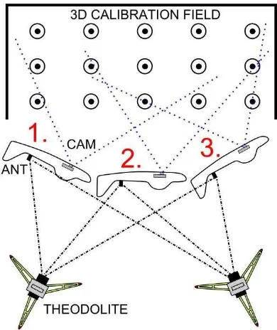
Spatial offset calibration, sometimes also called lever-arm calibration is rather complicated when the respective sensor centres are not known or not directly accessible. This is very often the case when using consumer grade cameras on unmanned aerial platforms. The antenna is located on the fuselage while the camera and an IMU are placed inside, Figure 4. Moreover, the centre of the camera sensor is not usually depicted on the camera body.
Therefore, an indirect estimation, such as “pseudo”- measurement technique has to be used (Ellum and El-Sheimy, 2002). These offsets are determined by building the difference in positions of GNSS antenna reference point determined by GNSS or tachymetry and origin of the camera frame resulting from a bundle adjustment. The lever-arm may be also estimated as an additional parameter when using precise observations of aerial position within bundle adjustment or within Kalman Filter (KF) for the case of antenna-IMU offset. However, accuracy of such estimation is somewhat limited because the spatial offset is correlated with the camera interior orientation parameters (Skaloud and Vallet, 2002), and respectively the accuracy of the velocity determination is not sufficient. In our case, we performed the pseudo measurement technique over a dedicated calibration field in a static scenario. The latter contains 25 GCPs determined with mm accuracy. The GCPs are located in a vertical and a horizontal planes constituting the 3D calibration field. The fuselage of the plane was mounted on a tripod in horizontal position with the camera pointing towards the calibration field as schematically shown in Figure 5. Then, the position of the antenna reference point (ARP) was measured by a theodolite from two stations. The theodolite was beforehand oriented to the local coordinate system. An image of the target field was taken by the camera and the process ISPRS Annals of the Photogrammetry, Remote Sensing and Spatial Information Sciences, Volume II-1/W1, 2015
repeated on the second and third camera stations. An additional set of 10 images was taken between stations 1 and 3 in order to establish a high number of tie-points and to better determine EO parameters of the camera at these stations. The processing was done in Pix4D mapper (Pix4D, 2015). The resulting camera EO parameters were further processed to express the spatial offsets between the camera perspective centre and ARP in the camera frame.
The short (i.e. 10 cm) lever arm between camera and R-IMU was measured by a calliper. Furthermore, the GNSS antenna L1 phase centre offset was determined by long observation with respect to an antenna with known parameters. The final calibrated 3D offset is 49 cm.
Figure 4. Schematic sketch of the sensor offsets between the camera instrumental frame, IMU-sensor frame and GNSS antenna
Figure 5. Schematic sketch (top view) of the sensor offsets calibration procedure; offsets measured from three stations
3.3 Angular Offsets
Considering the physical mounting of the IMU and the camera, a perfect alignment of these two systems is not possible. Similarly to the positional offset, the angular position of the IMU has to be determined with respect to the camera too. While the linear offsets between the different sensors can be measured with classical methods (by a calliper or by photogrammetry means) with millimetre accuracy, misalignment angles (also called boresight) cannot be determined this way with sufficient accuracy. A key assumption is that the boresight angles remain constant as long as the IMU remains rigidly mounted to the camera. This is very difficult to fulfil with standard off-the-shelf
components not originally foreseen to be used for mapping. There are several techniques of boresight calibration, for imaging sensors (Skaloud et al., 1996; Kruck, 2001; Cramer and Stallmann, 2002; Mostafa, 2002). Due to the employment of mass-market cameras, the calibration is thus not trivial and should be carried out regularly.
The boresight estimation can be done either within self-calibration adjustment (so-called one-step) or by comparing GNSS/INS derived attitude of images for which EO is estimated via (aerial position-aided) calibration block (so-called two-step procedure). The latter has the advantage of easier considering the remaining temporal correlations within the navigation system and leads to a realistic estimation of the variances (Skaloud and Schaer, 2003). The boresight misalignment was in our case calibrated during a calibration flight that is further described in the following sections.
3.4 Synchronization
The sampling of the IMU is performed within its firmware. The frequency is reset regularly by PPS (Pulse per second) provided by the GNSS receiver. The offset of entire second is determined by a time message recorded together with the IMU data by the FPGA board. As previously stated, the temporal synchronization between imaging and navigation sensor is assured by a flash pulse that the camera sends at the moment of shutter opening (Rehak et al., 2014). This can, however, cause small errors depending on the shutter speed. A half of the shutter speed duration is therefore considered to obtain an estimate of mid-exposure.
4. CASE STUDY
A case study was conducted over a dedicated calibration field that has the size of approximately 1 x 1.2 km. The terrain has height differences up to 30 m and includes a variety of surfaces such as crop fields, roads and forest. To asset the mapping accuracy, 26 dedicated markers were regularly placed across the field. The markers are permanently stabilized by surveying nails on tarmac, signalized by white colour circles and accurately surveyed.
4.1 Data Acquisition
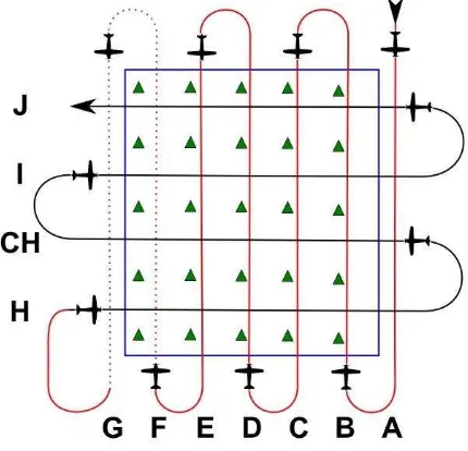
The presented test consists of three cases. The first case shows the integrated sensor orientation with aerial position control. The second case comprises the determination of the system calibration parameters. The third case deals with integrated sensor orientation in a narrow corridor. We would like to see if a pre-calibrated system together with GNSS/INS observations can ensure sufficient accuracy on the ground whilst the ground control points are completely taken out from the adjustment. The object space coordinate system of the whole test is Swiss LV95. The forward overlap was set to 80 %, the side overlap to 60 %. The composition of the flight is depicted in the
Figure 6. The strips from A to E and H to J served for the first and second cases. These two perpendicular strip configurations were executed in altitudes of 120 and 150 meters in order to better de-correlate IO/EO parameters. Two strips, F and G, representing a corridor, were excluded from the processing and ISPRS Annals of the Photogrammetry, Remote Sensing and Spatial Information Sciences, Volume II-1/W1, 2015
were exclusively used for the accuracy assessment. The length and width of the latter were 1200 m and 180 m respectively. The differences in topology of this particular corridor were around 30 m between the lowest and highest point. The average GSD was 3.8 cm/pixel.
Figure 6. An illustration of the executed flight
4.2 Data Processing
The processing pipeline was following that of classical airborne image processing. The flight resulted in a set of 520 images out of which 61 were used for the corridor evaluation. After the image acquisition, the images were processed in Pix4D mapper in order to obtain automatic image measurements of tie points and manual measurements of ground control and check points. The GNSS data were differentially processed in post-mission. Although the MAV is equipped with a modem for RTK corrections, post-processing allows better quality and more reliable assessment. The calculated antenna positions were subsequently fused in an Extended Kalman filter with 500 Hz IMU data for each IMU unit separately. The necessary sensor errors characteristic were obtained during a thorough calibration (Mabillard, 2013; Stebler et al., 2014). The resulted GNSS/INS positions of the IMU body were then translated to the camera instrumental frame while considering EO corrections for national mapping frame (Skaloud and Legat, 2006). At this stage, the boresight angles were considered as zero. The adjustment of image measurements with airborne position and attitude observations was performed within the standard photogrammetric suite Bingo (Kruck, 2001).
Same approach was used when processing the data from the second IMU. The difference between the respective boresight misalignments represent the relative orientation between the sensors inside the R-IMU. This is essential for combining their output by the foreseen type of processing in as synthetic-IMU, for details see (Waegli et al., 2008). It is worth noticing that the asset of R-IMU for noise reduction noticeably arises when employing more than just two IMUs simultaneously. Nonetheless, we used the synthetic IMU despite having just two sensors in order to evaluate the potential of such processing chain for further development.
5. RESULTS
5.1 Block with Aerial Position Control
We first focus our analysis on the achievable accuracy in block configuration where we adjust image observations together with aerial position observations while considering the IO parameters as unknown. We evaluated the mapping accuracy on 17 check points. No ground control points were used. The root-mean-square (RMS) of check point residuals is depicted in Table 1 and is 0.043 m horizontal and 0.040 m vertical, which corresponds in both directions approximately to 1 pixel. In Table 2 we show the mean of predicted accuracy of EO parameters for all images for indirect orientation (i.e. no position and/or attitude control). It should be noted that this accuracy is comparable with that of indirect sensor orientation using the current check points as ground control points.
Residual X [m] Y [m] Z [m]
MAX 0.069 0.053 0.059
MEAN 0.016 0.020 0.026
RMS 0.033 0.029 0.040
Table 1. Summary of the position accuracy at 17 check points
X [m] Y [m] Z [m]
0.013 0.020 0.018
Omega [deg] Phi [deg] Kappa [deg]
0.010 0.008 0.012
Table 2. Predicted accuracy of EO parameters
5.2 Self-Calibration
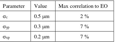
For de-correlating the IO/EO parameters and for estimating the boresight angles we run the adjustment of the block again, but this time with position and attitude observations. The coordinates of 17 signalized GCPs were introduced as weighted observations and the IO parameters and the boresight were considered as unknowns. The Table 3 summarizes the most pertinent results of the driving IO parameters. They are all estimated with reasonable accuracy, sufficiently de-correlated from EO and therefore can be fixed for the corridor project. The Table 4 highlights the quality of aerial position and attitude data. The aerial position and attitude residuals fulfil required accuracy of the GNSS/INS system. To highlight this further, Figure 7 depicts the achieved accuracy together with the influence of attitude errors on the ground for two different flying heights above ground. The estimated accuracies of omega a phi attitude angles can theoretically cause errors on the ground in 7 cm – 9 cm level. In the demonstrated example, it would represent an error of approximately 2 times the GSD.
Parameter Value Max correlation to EO
c 0.5 m 2 %
yp 0.3 m 7 %
xp 0.2 m 7 %
Table 3. Estimated precision of the camera parameters after self-calibration and their correlation to EO
X [m] Y [m] Z [m]
Aerial position residuals (RMS) 0.026 0.025 0.028
Maximum aerial position residuals 0.078 0.080 0.115
Omega
[deg] [deg] Phi Kappa [deg]
Aerial attitude residuals (RMS) 0.040 0.035 0.149
Maximum aerial attitude residuals 0.208 0.141 0.481
Table 4. Estimated accuracy of the GNSS/INS data
Figure 7. Propagation of roll and pitch errors on the ground from two different flying heights
5.3 Corridor mapping
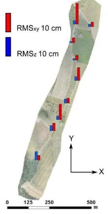
The previously estimated boresight angles were considered when transforming derived attitude for the two strips of our corridor. Adjustment using integrated sensor orientation was run twice with different configurations. In both cases, the IO parameters were fixed and no GCPs coordinates entered the adjustment. In the first case A, the adjustment was done with GNSS/INS derived positions only. In the second case B, the aerial positions and orientations were included. The results are summarized in Table 5 with respect to 9 independent check points which distribution is depicted in Figure 8.
In the case A, the insufficient lateral overlap causes noticeable errors in X component due to the absence of attitude control. The lack of GCPs degrades the accuracy of estimated image orientations that directly propagates on the ground. Systematic errors can be recognized by larger mean value which is in this case over 3 centimetres. Additionally, the position residuals are evidently higher with respect to the case B, except in the height component that is comparable.
In the case B, any significant mean value would indicate problems either in estimated IO parameters, wrongly calibrated offsets or a synchronization issue. However, values close to zero indicate that this is likely not the case. It can be seen that in all selected statistical indicators, the angular observations improved the results at independent check points. It can be clearly concluded that when having weak geometry of just two strips, as often the case of UAV corridor mapping, the angular observations play a major role in the final ground accuracy. Their contribution is mitigated (as shown in Table 1) in a strong block structure, while for single strip operations these observations become essential.
A
Residual X [m] Y [m] Z [m]
MAX 0.134 0.061 0.114
MEAN 0.035 -0.012 -0.008
RMS 0.059 0.033 0.070
B
MAX 0.051 0.035 0.136
MEAN 0.006 -0.007 -0.003
RMS 0.021 0.021 0.070
Table 5. Residuals at 9 check points, no GCPs used in the adjustment; A – position observations, B – position and attitude observations
The corridor was also processed in Pix4D mapper. Its current version (v.1.3) allows using aerial position control, hence possible orientation without GCPs. The measured attitude can be also introduced, however it does not contribute to the final mapping accuracy since the inputted values serve only as initial approximations. Therefore, the full potential of the described platform cannot be shown. Despite that, the directly measured attitude was used beforehand to correct the lever arm, thus it indirectly affects the positioning quality as well. Nevertheless, we aimed at testing the GNSS/INS derived positions in the state-of-the-art processing software that is dedicated to UAVs. The very same 9 check points were therefore used to assess the quality. In addition, the IO parameters were re-adjusted. As expected, the final residuals are slightly smaller in height, as shown in Table 6 and Figure 8, as some of the IO orientation parameters are correlated with those of EO. Re-adjusted IO can absorb some of the systematic effects. It shall be noticed, that although the maximal errors are similar to the second case of Table 5, the mean value is significantly higher in the Z component with respect to the previous cases. In order to clearly show the contribution of precise aerial control on the ground accuracy, several projects were calculated with a different approach to sensor orientation. Figure 9 shows ISPRS Annals of the Photogrammetry, Remote Sensing and Spatial Information Sciences, Volume II-1/W1, 2015
absolute height differences of resulted digital surface models (DSM) with respect to a reference model that was calculated from the entire block oriented by 26 GCPs in Pix4D mapper. It is obvious that the geometrical precision degrades with decreasing overlap on both sides of the corridor. There is little to no difference between the model oriented by 9 GCPs (case a) and the one oriented from the GNSS/INS observations (case c). On the other hand, when the distribution of GCPs is not favourable (case b), the accuracy degrades significantly in the absence of aerial control.
Residual X [m] Y [m] Z [m]
MAX 0.037 0.042 0.103
MEAN -0.015 0.016 0.047
RMS 0.022 0.025 0.049
Table 6. Pix4D – summary of the position accuracy at 9 check points
Figure 8. Corridor processed in Pix4D mapper with depicted residuals in position and height
6. CONCLUSION AND PERSPECTIVES
This paper introduced a fixed wing MAV and investigated the influence of in-flight measured exterior orientation parameters on ground accuracy in corridor mapping. The initial part discussed the problematic of sensor orientation with specific focus on corridor mapping, its difficulties and possible approaches. An in-house developed MAV platform was presented and tested during field missions. The imaging and navigation equipment carried on-board was introduced and calibrated. It consists of off-the-shelf components that were customized for the specific needs of MAV. Angular and spatial offsets were determined during separate calibration projects. Both are the prerequisites for accurate mapping based on integrated and/or direct sensor orientation using absolute EO control.
A case study was performed to calibrate the camera interior orientation parameters and boresight misalignment of employed R-IMU. A small corridor consisting of two parallel strips was selected and adjusted in two commercial software packages. Several processing strategies were tested with the conclusion that directly measured exterior orientation parameters can significantly improve ground accuracy while dropping the need for ground control establishment. It was shown that somewhat the low accuracy of measured attitude (with respect to much larger IMUs), which is in the level of 0.04 deg in roll and pitch, still considerably contributes in the aerial triangluation. The determination of the yaw angle is a challenge when using MEMS-based IMUs. The RMS of the latter was estimated to be 0.14 deg. On the other hand, given the fact that image angular orientation in yaw is mainly driven by forward overlapping images, the accuracy of yaw angle is somewhat less important. Nevertheless, this does not apply for direct sensor orientation where all the attitude angles are equally important.
The quality of synchronization and camera position control proved to be sufficient as the estimated aerial position accuracy lies in the level of 2 cm – 5 cm which corresponds to the kinematic accuracy of carrier-phase differential GNSS. The final RMS residuals in corridor evaluated at 9 independent check points lie at the level of 1 GSD in position and in the interval of 1.5-2 GSD in height.
In the case of processing in Pix4D mapper, the inclusion of precise observations of camera positions in MAV allowed to omit ground control points even in a project with weaker block geometry. Nevertheless, the absolute elimination of ground control points is usually not necessary and the corridor can start and end with a few control points to increase the redundancy and robustness. Nonetheless, with precise absolute position and attitude control, the need of ground control can be abolished especially inside the corridor.
The future development will be focused on testing of the R-IMU with higher level of redundancy. The performance of this unit is promising as indicated in this study and can further improve the accuracy of the camera orientation.
Figure 9. DSM differences with respect to the reference for different type of absolute orientation; a) 9 GCPs, b) 4 GCPs, c) accurate GNSS/INS positions
REFERENCES
Ardupilot, 2015. Mission Planner [WWW Document]. URL http://planner.ardupilot.com/ (accessed 3.26.15).
Colomina, I., 1999. GPS, INS and Aerial Triangulation: what is the best way for the operational determination of photogrammetric image orientation? Presented at the ISPRS Conference Automatic Extraction of GIS Objects Digital Imagery, München, Germany.
Colomina, I., 2007. From Off-line to On-line Geocoding: the Evolution of Sensor Orientation. Photogrammetric Week’07, Wichmann, Germany.
Colomina, I., Molina, P., 2014. Unmanned aerial systems for photogrammetry and remote sensing: A review. ISPRS Journal of Photogrammetry & Remote Sensing 92, 79–97.
Cramer, M., Stallmann, D., 2002. System Calibration for Direct Georeferencing, in: Photogrammetric Computer Vision, ISPRS Commission III Symposium. Graz, Austria, p. 6.
Delair-Tech, 2014. Power Lines Inspections Using MINI-UAV. Presentation, Madrid, Spain.
Ellum, C., El-Sheimy, N., 2002. Inexpensive Kinematic Attitude Determination from MEMS-Based Accelerometers and GPS-Derived Accelerations. NAVIGATION: Journal of the Institute of Navigation 49, 117–126.
Fraser, C.S., 1997. Digital camera self-calibration. ISPRS Journal of Photogrammetry and Remote Sensing 52, 149–159.
Heipke, C., Jacobsen, K., Wegmann, H., 2002. Integrated Sensor Orientation. OEEPE Official Publication 43.
Intersense, 2012. NavChip [WWW Document]. URL http://www.intersense.com/pages/27/227/ (accessed 3.20.15).
Jacobsen, K., 2004. Direct/Integrated Sensor Oerientation - Pros and Cons. Presented at the XXXV ISPRS Congress, International Archives of the Photogrammetry, Remote Sensing and Spatial Information Sciences, Istambul, Turkey, pp. 829– 835.
Javad, 2015. [WWW Document]. URL
http://www.javad.com/jgnss/ (accessed 3.26.15).
Kluter, T., 2012. GECKO4NAV Technical Reference Manual Revision 1.0.
Kruck, E., 2001. Combined IMU and sensor calibration with BINGO-F, in: Integrated Sensor Orientation, Proc. of the OEEPE Workshop ". CD-ROM, Hannover, pp. 84–108.
Lichti, D., Skaloud, J., Schaer, P., 2008. On the calibration strategy of medium format cameras for direct georeferencing, in: International Calibration and Orientation Workshop EuroCOW 2008.
Mabillard, R., 2013. Sensor Orientation with Gecko4Nav RIMU (Master Thesis). École Polytechnique Fédérale de Lausanne, Lausanne, Switzerland.
MAVinci, 2015. MAVinci - Unmanned Aerial Systems [WWW Document]. URL http://www.mavinci.de/ (accessed 3.26.15).
Maxtena, 2014. Maxtena [WWW Document]. URL http://www.maxtena.com/ (accessed 3.20.15).
Meier, L., Tanskanen, P., Heng, L., Lee, G.., Fraundorfer, F., Pollefeys, M., 2012. PIXHAWK: A micro aerial vehicle design for autonomous flight using on-board computer vision. Autonomous Robots 33, 21–39.
Modellsport GmbH, 2015. Multiplex [WWW Document]. URL http://www.multiplex-rc.de/en.html
Mostafa, M., 2002. Camera/IMU boresight calibration: New Advances and performance analysis, in: ASPRS Annual Meeting. Washington, DC, USA.
Pix4D, 2015b. Pix4Dmapper [WWW Document]. URL http://pix4d.com/ (accessed 3.27.15).
Rehak, M., Mabillard, R., Skaloud, J., 2014. A micro aerial vehicle with precise position and attitude sensors. Photogrammetrie, Fernerkundung, Geoinformation (PFG) 4, 239–251. doi:10.1127/1432-8364/2014/0220
Schwarz, K.., Chapman, M.., Cannon, M.., Gong, P., 1993. An integrated INS/GPS approach to the georeferencing of remotely sensed data. Photogrammetric Engineering & Remote Sensing 59, 1667–1674.
senseFly, 2015. Drones vs traditional instruments: corridor mapping in Turkey.
Skaloud, J., Cramer, M., Schwarz, K.P., 1996. Exterior orientation by direct measurements of camera position and attitude. International Archives of Photogrammetry, Remote Sensing and Spatial Information Sciences 31, 125–130.
Skaloud, J., Schwarz, K.P., 2000. Accurate orientation for airborne mapping systems. Photogrammetric Engineering and Remote Sensing 66, 393–401.
Skaloud, J., Vallet, J., 2002. High accuracy handheld mapping system for fast helicopter deployment, in: Joint International Symposium on Geospatial Theory, Processing and Applications, ISPRS Comm. IV. Ottawa, Canada.
Skaloud, J., Schaer, P., 2003. Towards a More Rigorous Boresight Calibration. Presented at the ISPRS International Working Shop on Theory, Technology and Realities of Inertial / GPS Sensor Orientation, Castelldefels, Spain.
Skaloud, J., Legat, K., 2006. CAMEO - Camera exterior orientation by direct georeferencing. EPFL TOPO, Lausanne, Switzerland.
Skaloud, J., 2006. Reliability of direct georeferencing phase 1: An overview of the current approaches and possibilities, in: Checking and Improving of Digital Terrain Models / Reliability of Direct Georeferencing. EuroSDR Official Publication 51.
Stebler, Y., Guerrier, S., Skaloud, J., Victoria-Feser, M.-P., 2014. The generalized method of wavelet moments for inertial navigation filter design. IEEE Transactions on Aerospace and Electronic Systems 50, 2269–2283.
Syed, Z.P., P Aggarwal, Goodall, C., Niu, X., El-Sheimy, N., 2007. A new multi-position calibration method for MEMS inertial navigation systems. Measurement Science and Technology 18, 1897–1907.
Waegli, A., Guerrier, S., Skaloud, J., 2008. Redundant MEMS-IMU integrated with GPS for performance assessment in motorsports, in: PLANS 2008 - Joined Symposium of IEEE and ION on Position Location and Navigation.
Waegli, A., Skaloud, J., Guerrier, S. Pares, M.E., 2010. Noise reduction and estimation in multiple micro-electro-mechanical inertial systems. Measurement Science and Technology 21, 065201–065212.