isprs archives XLII 2 W4 135 2017

FITTING A POINT CLOUD TO A 3D POLYHEDRAL

SURFACE

Eugene Vladimirovich Popova,∗_{, Serge Igorevich Rotkov}a a _{Engineering Geometry and Computer Graphics Chair} Nizhegorodsky State Architectural and Civil Engineering University,

603950, 65, Ilyinskaya Street, Nizhny Novgorod, Russia popov_eugene@list.ru

Commission II, WG II/10

KEYWORDS: Contactlessmeasurement, point clouds fitting, Stretched Grid method, Principal Component Analysis ABSTRACT

The ability to measure parameters of large-scale objects in a contactless fashion has a tremendous potential in a number of industrial applications. However, this problem is usually associated with an ambiguous task to compare two data sets specified in two different co-ordinate systems. This paper deals with the study of fitting a set of unorganized points to a polyhedral surface. The developed approach uses Principal Component Analysis (PCA) and Stretched grid method (SGM) to substitute a non-linear problem solution with several linear steps. The squared distance (SD) is a general criterion to control the process of convergence of a set of points to a target surface. The described numerical experiment concerns the remote measurement of a large-scale aerial in the form of a frame with a parabolic shape. The experiment shows that the fitting process of a point cloud to a target surface converges in several linear steps. The method is applicable to the geometry remote measurement of large-scale objects in a contactless fashion.

∗

_{Corresponding author}

1. INTRODUCTION

The geometry measurement of large-scale objects in any industry is a very acute problem. It reduces to the comparison of a 3D point set given by remote measurement to a continuous theoretical surface. We can classify it as a point-to-surface (PTS) problem. Usually one can treat such comparison as superposition that requires not less than three reference points. However, reference points can be either unknown or meaningless for some classes of product. In this case, the problem comes to a comparison of two geometric objects in 3D space according to a given criterion of optimality. That is, the unknown parameters of the 3D transformation such as translation and rotation are a subject to be found according to objects optimal matching.

All the algorithms of two 3D sets comparison can be classified in the following way:

1. ICP- algorithm (iterative closest point algorithm). The basis of ICP-algorithm is the assumption that two objects have common area where they coincide well enough. It means that in the common area, for both of them, each point of one object has a corresponding point of another object. Vaillant and Glaunes (Vaillant at al., 2005.) described the basics of the ICP-algorithm. Though some disadvantages of ICP-algorithm take place:

- the computational complexity of the closest points finding is

O(mN1 N2) where m - number of iterations, N1- number of the first object points, N2 - number of the second object points (Friedman , at al. 1977);

- strong dependence on the given initial approximation; - strong dependence on the density of point clouds;

- the method requires the existence of a large overlap region where the points of one cloud correspond to the points of another cloud.

Recently, many variants of the original ICP approach have been proposed, such as:

- Brunnstrom and Stoddart (Brunnstrom, at al.1996) describe the genetic algorithm of finding the most successful initial approximation which is input data to ICP-algorithm;

- the research of Dyshkant (Dyshkant, 2010) is also dedicated to the ICP-algorithm modification based on the k-d trees, which allows minimization of the computational complexity to O(mN1 logN2);

- in works of Liu, Li, and Wang (Y. Liu, at al. 2004) algorithms to improve the accuracy and reliability of the ICP-algorithm by imposing certain restrictions of the input data are proposed. 2. Methods based on curvature maps.

This class of methods requires knowledge of the curvature of the surface given by the point cloud. The algorithm was described by Gatzke at al. (Gatzke, at al., 2005). The disadvantage of this method is a strong dependence on the point cloud density because it affects the accuracy of the curvature calculation.

3. Other methods.

The authors of (Bergevin, at al. 1995) describe the algorithm that does not require the approach of initial data. This algorithm can use a free-form surface; however, it has a very low speed. The authors of work (Sitnik, at al. 2002) improved the method of the steepest descent optimization. The disadvantage of the approach is the quadratic computational complexity.

Delaunay triangulation algorithm in combination with Nelder-Mead method are described in works (Dyshkant, 2010) and (Nelder, at al.1965). The algorithm assumes that the surfaces are single-valued. This algorithm as well as ICP-algorithm depends on the given initial approximation.

The authors of (Gruen, at al. 2005) proposed the algorithm based on the least square method. The algorithm requirement is that the point clouds have a significant overlap area.

Nowadays there are two trends in the surface superpose problem solution. The first group of methods limits the initial data therefore they work fast. The second group is more general but has a large computational complexity. Hence, we need more algorithms for the comparison of the two data sets.

2. INITIAL BACKGROUND

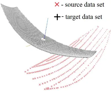
The initial assumption is that there are two sets:

P:P

i

(x

i

,y

i

,z

i

)

–

the cloud of source points obtained by measuring and )

(x_i,y_i,z_i i P :

P – the cloud of target points (see Fig. 1). We should fit point cloud P to a target point cloud P.

Figure 1: Two data sets

However, we cannot make it directly because of the lack of definite and understandable base points. Besides, both data sets have different structure so there are no corresponding points to compare. Therefore, we triangulate a target cloud and turn it into a continuous 3D polyhedral surface

Σ

(see Fig.2) specified on the same bounded domain

D

⊂

R

2

_{as a target data set. It is}

required to find such

Ω

opt transformation amongst all possible

Ω

3D transformations so that the source set

Ω

opt

(

P

) could be in

closest state to the surface

Σ

according to the given distance function

ρ

. That is

( )

(

)

_∑

(

( )

)

∑

= Ω =

Ω Σ =

Ω

Σ N

i

i N

i

i

opt P P

1 1

, min

,

ρ

ρ

(1)

where

ρ

(Σ,

X

) - the distance function from point

X

to surface

Σ

.

Once the two sets are specified with respect to two different origins we need such transformation of one of them as ‘rigid body’ so that to ensure the satisfaction of the eqn (1). Such 3D transformation is defined by six parameters: the components of the translation vector

Δ

x

c

,Δ

y

c

,Δ

z

c (here C is the geometry

center of relocatable set) and three rotation angles

φ

x

, φ

y

, φ

z,.

The numerical solution of this non-linear problem by the usual optimization approaches is very complicated for various reasons, namely:

• In general, it is difficult to fit two sets even approximately. Hence, it is impossible to find the initial values of

Δ

x

c

,Δ

y

c

,Δ

z

c

, φ

x

, φ

y

, φ

z. It forces us to take them with

maximum values that makes the computing process slow down.

• The surface cannot be simply single coherent that increases the number of constraints in the optimization problem.

• Often the surface does not have analytical representation, so its derivatives are unknown or do not exist. That makes it impossible to use efficient numerical algorithms based on the function derivatives.

• The computation time depends on value

N

(the number of points in

P

set). Therefore, the computing process becomes very slow when the dense of the point set grows significantly.

Figure 2: The source data set and the 3D surface Taking it into account we propose a new approach that consists of two stages and the first of them is Principal Component Analysis (PCA). We apply PCA to the so-called ‘rough fit’ that actually is the approximate initial fit of two sets. The second stage is the precise fit based on Stretched grid method (SGM) that allows accurate fitting of two sets according to minimum SD criterion in 1-4 linear steps. We demonstrate this approach with the help of the parabolic aerial where

Σ

–

analytic aerial surface,

P

–

source point cloud obtained by measuring the aerial with the standard electronic tacheometer «Trimble-M3» (Survey of Trimble M3 Mechanical Total Station). Thus, the target data set was obtained on the basis of available documentation.

3. ROUGH FIT

It should be noted, that PCA is often used to map data on a new orthonormal basis in the direction of the largest variance (Draper, at al., 2002). The largest eigenvector of the covariance matrix always points to the direction of the largest variance of the data.

covariance matrices are calculated. The largest eigenvector is a vector in the direction of the largest variance of the 3D point cloud, and therefore, represents the point cloud’s rotation. Further, let A be the covariance matrix, let v be an eigenvector of this matrix, and let

λ

be the corresponding eigenvalue. The problem of eigenvalues decomposition is then defined as

Ax = λx

,

(2)

and further reduces to

x

(

A − λI

) = 0.

(3)

It is clear that (3) only has a non-zero solution if

A − λI

is singular, and consequently if its determinant equals to zero

det

(

A − λI

) = 0

.

(4)

The eigenvalues can simply be obtained by solving (4), whereas the corresponding eigenvectors are obtained by substituting the eigenvalues into (2). Once the eigenvectors are known for each point cloud, the fit is achieved by aligning these vectors. Then, let us assume that matrix TΣ represents the transformation that would align the largest eigenvector of the target point cloud related to surface

Σ

with the X-axis. Now, let us suppose that matrix TP represents the transformation that would align the

largest eigenvector of the source point cloud P with the X-axis as well. Finally, we can align the source point cloud with the target point cloud easily if we take into account coincidence of both principal component systems (Xpr

,

Y

pr

,

Z

pr) of source

and target point clouds (see Fig.3).

Figure 3: Two data sets in common principal component system

Here we face some disadvantage, as we cannot always determine the direction of collinear principal component axes uniquely with PCA (see Fig.3). Therefore, we correct their directions in this issue manually by rotating the source point cloud about axes Xpr

,

Y

pr

,

Z

pr consequently to meet the

minimum of SD criterion. In our sample, we rotate the point cloud about

X

pr (see Fig. 4.)

The rough fit cannot obtain real minimum solution according to the SD criterion; therefore, the next stage is the precise fit.

4.PRECISE FIT

The precise fit stage is based on SGM. SGM described in work (Popov E.V., 1997) is a numerical technique for finding approximate solutions of various mathematical and engineering problems that can be related to an elastic grid behavior. In our case, we apply SGM to drag in the source point cloud as a ‘rigid body’ to the target surface by the set of elastic springs (Fig.5).

Figure 4: The rough fit of two data sets in common principal system

Figure 5. The precise fit scheme

Each elastic spring for our cloud connects the nearest neighbor point on the target surface qi of each point pi in the source point

cloud (see Fig. 5). We find the neighbor point on the target surface by normal projection of the source point onto the target surface. This approach is similar to ICP point-to-point technique described in (Ben Bellekens, at al. 2014) but is much easier and has another physical meaning.

The aim of the precise fit is to find functions

Δ

x

c

,Δ

y

c

,Δ

z

c

, φ

x

,

φ

y

, φ

z that obtain the minimum to exp (1). If we apply classical

motion equation, we should further resolve non-linear equation system consisted of transcendental functions. The advantage is that we can consider linear dependence of displacement of points on the cloud rotation as a rigid body (see Fig. 6).

Figure 6: To rigid body rotation and transformation

Taking into consideration the ‘rigid body’ rotation of point cloud due to precise fit, we can write the displacement of an arbitrary point pi (Fig.6) as follows

    

    

∆ ∆ ∆ +     

    

∆ ∆ ∆

  

 

  

  =     

    

∆ ∆ ∆

c c c

j j j

i i i

i i i

i i i

i i i

z y x

z y x

B B B

B B B

B B B

z y x

) ( 33 ) ( 32 ) ( 31

) ( 23 ) ( 22 ) ( 21

) ( 13 ) ( 12 ) ( 11

where

Δ

x

i

,Δ

y

i

,Δ

z

i – displacements of an arbitrary point i;

Δ

x

j

,Δ

y

j

,Δ

z

j – displacements of point j;

Δ

x

c

,Δ

y

c

,Δ

z

c - displacements of the point cloud centroid.

We can calculate the components of the normalized matrix B

for an arbitrary point of the cloud as a rotation matrix about the unit vector s(u,v,w) at the angle θ (see Fig. 6) by the following

respectively from the point cloud centroid.

Due to exp (5) we can calculate the displacement of each point in the point cloud if we know the displacement of single point number j only.

The further step is to write the expression for the potential energy of entire connecting lines between the cloud points and the springs including (Fig. 4) that takes the following form

∑

Then, let us assume that co-ordinate vector {X} of all the points of the cloud is associated with a final cloud position, when the source cloud is fit to the target surface and the vector {X}' is associated with the initial point cloud position. Thus, vector {X} will look in the following way

To determine vector {∆X} we should derive function (7) by incrementing vector {∆X} with form (8) taken into account, i.e.

0

t - number of the current co-ordinate.

After transformations using exps (5), (7), (8), (9) and keeping all lengths

L

ij constant (see Fig.6) we can obtain the following

linear equation system 6×6

K·Δx = Q, (10)

{

( ) ( ) ( )

}

,

1

) ( 33 )

( 23 )

( 13

3=∑ − + − + −

=

n

i

i j i i j i i j i

z z B y y B x x B Q

, 4 xj

Q =

, 5 yj

Q =

, 6 zj

Q =

When all six unknown functions

Δ

x

j

,

Δ

y

j

,

Δ

z

j

,

Δ

x

c

,

Δ

y

c

,

Δ

z

c

are found we can calculate displacement of each source point due to precise fit using exp (5).

5.“SURFACE FITTING” PROGRAM

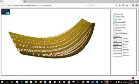
We developed the program named “Surface Fitting” based on the above described algorithm (Popov, 2016). To make the program extremely accessible and mobile we developed it as a web-based open source application using JavaScript language (Flanagan, 2011) in couple with THREE.JS library (Dirksen, 2013). As it is known, JavaScriptis an object-oriented language designed in 1995 to allow non-programmers to extend web sites with client-side executable code. The language is also becoming a general-purpose computing platform with office applications, browsers and development environments being developed in JavaScript. Unlike other traditional languages such as Java, C++ or C#, JavaScript strives to maximize programming flexibility and is ideal for programming accessible applications including portable measuring systems. THREE.JS is a high-level, scene graph framework for 3D graphics built on top of WebGL. THREE.JS programs are written in JavaScript because there is no alternative for WebGL. The main idea when creating the program was to provide the user with a simple, accessible tool that depends neither on the hardware nor on the software platform. In Fig.7 one can see the user interface of the “Surface Fitting” program.

Figure 7: User interface of “Surface Fitting” program.

Using “Surface Fitting” program we can calculate the displacements of entire source points to fit it to the target surface and visualize the whole scene. Input data in the form of source and target point clouds are loaded into the program automatically. The process involves four consecutive steps

• target cloud triangulation,

• rough fit,

• source cloud rotation about principal axes manually at

π

-angle if necessary

• and the final precise fit.

In spite of linear nature of the precise fit, the process needs some iterations to converge because of some disparity of two

sets after rough fit. Table 1 shows the matching error of SD against the number of iterations.

Iterations Relative Error of SD,% Time, sec 2 In spite of linear nature

4.64

8 1.5257 18.30

17 0.0984 46.72

20 0.0107 55.00

29 0.0064 85.55

Table 1: The process convergence

The final fit of two sets can be seen in Fig.8.

Figure 8: The final fit of two data sets.

As we can see, the process meets minimum SD criterion very quickly. The final error (about 0.01%) means that the fit precision is about 1-2 mm for the aerial with about 15m of overall dimension.

6. CONCLUSION

This paper has introduced a new two-stage method based on rough fit with PCA and precise fit by SGM for direct point cloud and polyhedral surface fit in 3D. The algorithm has been designed for accurate distance minimizing between source and target data sets. It differs from techniques based on the ICP-algorithm and it differs from any Least Square approaches due to clear physical meaning. It does not depend on the configuration of data sets and their connectivity. The method consists of several linear steps and converges very fast. By vary the residual criterion, we can achieve any level of the fitting relative error.

The “Surface Fitting” allows calculation of both data sets at the initial and fitting position. It also provides the user with comprehensive and detailed tools of the whole scene visualization.

The only temporary inconvenience in using this method for 3D data sets comparison is the ambiguity of transformations with a rough fitting when applying PCA. We are currently resolving this problem by simple manual correction consequentially rotating the source data set at

π

-angle about principal axes to obtain local SD minimum. In the future, we plan to make it automatic. Besides, we intend to improve PCA algorithm by making it less sensitive to the data set singularities.

be aligned accurately with a set of 3D measurements. Such applications are cancer-tissue detections, hole detection, dental occlusion modelling, artefact recognition, etc.

7. AСKNOWLEDGMENTS

Russian Foundation for Basic Research has supported this work under grant # 15-07-01962 and grant # 15-07-05110.

REFERENCES

Vaillant M . , Glaunes J.,2005. Surface matching via currents.

Lecture Notes in Computer Science: Information Processing in Medical Imaging — Vol. 3565. - Pp. 1-5

Friedman J., Bentley J.L., Finkel R.A., 1977. An Algorithm for Finding Best Matches in Logarithmic Expect.ed Time. ACM Transactions on Mathematical Software. - Vol.3, no.3.-pp. 209-226

Brunnstrom K., Stoddart A. J., 1996. Genetic algorithms for free-form surface matching Proc. ICPR. - pp. 689-693.

Dyshkant N., 2010 An algorithm for calculation the similarity measures of surfaces represented as point clouds. Pattern Recognition and Image Analysis: Advances in Mathematical Theory and Applications -Vol.20, no.4-Pp. 495-504.

Y. Liu, L. Li, and Y. Wang, 2004. Free Form Shape Matching Using Deterministic Annealing and Softassign, in 17th International Conference on Pattern Recognition, Cambridge, United Kingdom, August 23-26.

Y. Liu, L. Li, and B. Wei, 2004. 3D Shape Matching Using Collinearity of Constraint, in IEEE International Conference on Robotics and Automation, New Orleans, LA, April 26 - May 1.

Gatzke T., Zelinka S., Grimm C., Garland M., 2005. Curvature Maps for Local Shape Comparison. In: Shape Modeling International. — Pp. 244-256

Bergevin, R., Laurendeau, D., Poussart D., 1995. Registering Range Views of Multi-Part Objects, Computer Vision and Image Understanding. IEEE Trans. Pattern Analysis and Machine Intell., 61(1):1–16, Jan.

Sitnik R., Kujawinska M., 2002. Creating true 3d-shape representation merging methodologies. Three-Dimensional Image Capture and Applications V, Proceedings of SPIE Vol. 4661, pp. 92-99.

Nelder J.A., Mead R., 1965. A simplex method for function minimization. Computer Journal. - Vol. 7. Pp. 308-313

Gruen A., Akca D.,2005. Least Squares 3D Surface and Curve Matching. ISPRS Journal of Photogrammetry and Remote Sensing. — Vol. 59. — Pp. 151-174.

Popov E.V., Rotkov S.I. , 2013. The Optimal Superpose of a Finite Point Set With a 3D Surface, Proceedings of the International Conference on Physics and Technology CPT2013, 12-19 of May 2013, Larnaca, Ciprus

Survey of Trimble M3 Mechanical Total Station, http://www.trimble.com/Survey/trimblem3.aspx

B. Draper, W. Yambor, and J. Beveridge, 2002. Analyzing PCA-based face recognition algorithms: Eigenvector selection and distance measures, Empirical Evaluation Methods in Computer Vision, pp. 1–14.

Ben Bellekens, Vincent Spruyt, Rafael Berkvens, and Maarten Weyn, 2014. A Survey of Rigid 3D Point cloud Registration Algorithms, AMBIENT 2014: The Fourth International Conference on Ambient Computing, Applications, Services and Technologies, IARIA, pp. 8–13.

Popov E.V., 1997. On Some Variational Formulations for

Minimum Surface. Transactions of Canadian Society of Mechanics for Engineering, Univ. of Alberta, vol.20, N 4, pp. 391–400.

Popov E.V., 2016. “Surface Fitting”, The State Certificate # 2016661441 of computer program, Federal Service of intellectual property, Russian Federation.

Flanagan, David, 2011. JavaScript: The Definitive Guide (6th ed.). O'Reilly & Associates. ISBN 978-0-596-80552-4.