REAL AND SIMULATED WAVEFORM RECORDING LIDAR DATA IN BOREAL
JUVENILE FOREST VEGETATION
A. Hovi, a, *, I. Korpela a
a Department of Forest Sciences, POB 27, 00014 University of Helsinki, Finland - (aarne.hovi, ilkka.korpela)@helsinki.fi
KEYWORDS: Radiative transfer modeling, LiDAR, Waveform, Monte Carlo ray tracing, Simulation, Vegetation structure
ABSTRACT:
Airborne small-footprint LiDAR is replacing field measurements in regional-level forest inventories, but auxiliary field work is still required for the optimal management of young stands. Waveform (WF) recording sensors can provide a more detailed description of the vegetation compared to discrete return (DR) systems. Furthermore, knowing the shape of the signal facilitates comparisons be-tween real data and those obtained with simulation tools. We performed a quantitative validation of a Monte Carlo ray tracing (MCRT) -based LiDAR simulator against real data and used simulations and empirical data to study the WF recording LiDAR for the classification of boreal juvenile forest vegetation. Geometric-optical models of three common species were used as input for the MCRT model. Simulated radiometric and geometric WF features were in good agreement with the real data, and interspecies differ-ences were preserved. We used the simulator to study the effects of sensor parameters on species classification performance. An increase in footprint size improved the classification accuracy up to a certain footprint size, while the emitted pulse width and the WF sampling rate had minor effects. Analyses on empirical data showed small improvement in performance compared to existing stud-ies, when classifying seedling stand vegetation to four operational classes. The results on simulator validation serve as a basis for the future use of simulation models e.g. in LiDAR survey planning or in the simulation of synthetic training data, while the empirical findings clarify the potential of WF LiDAR data in the inventory chain for the operational forest management planning in Finland.
1. INTRODUCTION
The capability of small-footprint airborne LiDAR in produc-ing precise estimates of quantitative forest characteristics is well demonstrated (Naesset et al., 2004). A direct outcome has been the replacement of traditional field-based inventory methods (Maltamo et al., 2011). In Finland, airborne LiDAR, combined with aerial images, is used in regional level inven-tories for operational forest management planning. Currently, the inventory of seedling stands is a separate process in the field. It would be beneficial, if the wall-to-wall remote sens-ing (RS) data could be utilized in seedlsens-ing stands also. The most important variables sought are the need and timing of silvicultural treatments (weed, insect, and herbivore control, clearing to favor the future trees).
Pulsed LiDAR systems send 5–10-ns long, collimated beams of laser light towards the target at high frequency. The return-ing signal is a convolution of the time-dependent function of the transmitted pulse power with the target cross-section profile and the system response function (Wagner et al., 2006). Discrete-return (DR) sensors detect echoes from the returning pulse (range detection) on-the-fly. Coordinates and an intensity measurement are delivered for each echo. Wave-form (WF) recording systems store a digitized amplitude sequence, the waveform, for post processing (Blair et al., 1994). It is evident that WF data provide a more accurate characterization of vegetation. Research of WF data in forest applications has focused on deriving more dense point clouds by finding additional echoes, or on using radiometric WF features for classification tasks.
Operational area-based forest inventories rely on empirical dependencies established between the forest variables and LiDAR metrics (Packalén and Maltamo, 2007). Theoretical simulations, although not completely replacing the need for empirical training and validation data, can be useful in e.g. studying the effects of acquisition settings on the observed LiDAR signal, or in the planning of sampling strategies. In
addition, simulations allow for testing interpretation algo-rithms and extending the empirical results. In theory, it is also possible to predict forest variables from the LiDAR data through the inversion of the simulation model, i.e. to produce synthetic training data. Comparison against real data is essen-tial to verify the correctness of the simulation models, and to test their robustness to various parameters and assumptions. From the validation point of view, DR systems are ‘black boxes’, whereas in WF systems, the shape of the returning signal is observed, which facilitates comparisons between simulated and real data. Recent studies demonstrate the use of Monte Carlo ray tracing (MCRT), combined with explicit leaf- or needle-level vegetation models in simulation of opti-cal RS signals (e.g. Disney et al., 2006). The MCRT is con-sidered as one of the most accurate methods for radiative transfer modeling in vegetation (Widlowski et al., 2008). There have been applications to LiDAR as well (Disney et al., 2010; Morsdorf et al., 2009), but comparisons to real data are often lacking.
We developed a MCRT simulation model for WF recording LiDAR data. The overall aims of our study were related to the validation of the model and to the examination of the potential of WF data in the mapping of seedling stand vegeta-tion. Three specific research aims (RA) were formulated:
RA1) To perform quantitative validation of the simulation model against real data and test the model sensitivity to vege-tation parameters.
RA2) To use the simulation model for testing the effects of different sensor parameters on the performance of WF data in the classification of three selected plant species.
2. MATERIALS AND METHODS
2.1 Field reference
The field data in Hyytiälä, Finland (61°50 N, 24°20 E), were collected in the summers of 2010 and 2012. Seedling stands were chosen to represent variation in stand age and site type (Figure 1). Average tree height was 1.5–5 m, but some re-cently established stands were selected also for sampling of low vegetation. A vegetation sample refers to a tree or a circular area containing low vegetation. The tree base or the ground at the center of the circle was positioned in 3D with Network GNSS at an accuracy of better than 3 cm. Two types of sampling schemes were used. In 2010, rectangular plots (100–200 m2) were established at subjectively selected loca-tions. All trees were positioned and recorded for height and species. Both in 2010 and 2012, separate vegetation samples were collected. The samples include trees and circular sam-ples of low vegetation (r = 0.5 m in 2010, r = 1.0 m in 2012). Maximum height was measured for each sample. A subjec-tive estimate of the leaf cover (0–100%) was recorded for a subset of the 2012 samples.
Figure 1. Examples of the selected stands. A 12-year-old sowed pine stand on a barren site (left), and a 11-yr-old planted spruce with a naturally regenerated broadleaved mixture on a fertile site (right).
2.2 LiDAR data
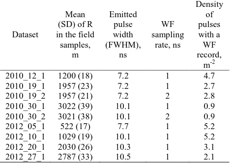
Data from two Leica ALS60 campaigns (15–17 GMT, July 19, 2010 and 17–19 GMT, July 5, 2012) were used. The data include nine datasets differing by acquisition height and WF sampling rate (Table 1). The ALS60 sensor operates at of 1064 nm. The beam divergence is 0.15 mrad at 1/e, and 0.22 mrad at 1/e2. Up to four DR echoes can be recorded per pulse. An echo consists of target coordinates, and eight-bit values for the intensity and the automatic gain control (AGC). The returning signal is directed to a separate WF sampling unit, and the first DR echo detected triggers the WF recording. The continuous 256-ns-long (38 m) WF record contained a sample of 5 m that preceded the first echo. Max-imum scan zenith angle was always 15°. The WF data were recorded for every pulse, except in the datasets of 2010_12_1 and 2012_05_1 in which every second pulse pair was record-ed due to data transfer constraints. In the 2012 campaign, the peak power of the pulses was adjusted for constant irradiance at the ground from all four acquisition heights. Campaign-level boresight and range calibrations were carried out fol-lowed by relative strip matching for correcting the roll, pitch and height discrepancies. The trajectory data was also availa-ble, giving the 3D pulse vector.
ALS60 applies the AGC that regulates the receiver gain. To account for AGC effects on the signal level, we used a nor-malization model: parameter a is a reference AGC value to which raw values are normalized, and parameter b gives the increase in signal level per unit increase of AGC. The model was applied to the WF data by replacing Ical and Iobs with the amplitude values, and the whole WF sequence (excluding noise) was then normalized using Eq. 1. The value of parameter a was set at the average AGC value in each dataset, and optimal values for b were searched for by minimizing the nested coefficient of variation (CV) of the WF peak amplitude data, using homogeneous targets, which covered a range of surface reflectivity. Because of small range (R) deviation within the datasets, no R normalization was applied.
Table 1. Overview of the LiDAR datasets.
Dataset
2.3 The simulation model
MCRT simulation: MCRT was used for estimating the ratio
of scattered radiant intensity towards the receiver [W sr-1] to the incident irradiance at target surface [W m-2] i.e. the dif-ferential scattering cross-section of the target ( , [m2 sr-1]).
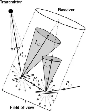
Our model works in forward mode i.e. the photon paths (rays) are traced from the light source (Gaussian beam) to the receiver (Figure 2). For input, geometric-optical representa-tion of the scene i.e. the coordinates and orientarepresenta-tions of the scene elements as well as their reflectance ( ) and transmit-tance ( ) are required. The model solution calls for finding intersections of the rays with the scene elements, for which bi-Lambertian scattering properties are assumed. If the re-ceiver is visible from an intersection point, the contribution of ray i of scattering order n to the total radiant intensity towards the receiver (Ii,n) is calculated from the , view-zenith angle ( ) in relation to surface normal, and the incident power of the ray (Pi,n-1):
Figure 2. Illustration of the MCRT sampling scheme. The dashed small arrows represent the populations of all possible photon paths that are sampled. Note that in reality the receiv-er and transmittreceiv-er are at the same location in LiDAR sensors.
By setting the total power of the emitted rays at 1, the output from the MCRT is directly the target . To account for the time-dependency of the LiDAR signal, was binned into 0.05-ns-long intervals (cross-section profile, (t)) based on the lengths of the individual ray paths. We used 30000 rays per pulse and 10 scattering orders in the simulations.
Convolution with system WF: To obtain the voltage pattern
recorded by the instrument, the LiDAR system WF was convoluted with the simulated (t) (Eq. 7). The formula is derived as follows. The instrument emits light at power Pe(t) [W]. The instantaneous irradiance at target [W m-2] is ob-tained by multiplying Pe(t) with the atmospheric attenuation factor ( atm, [unitless]) and by dividing with the target surface area (A, [m2]). The radiant intensity towards the receiver (I(t), [W sr-1]) is then the convolution of the irradiance with (t)
The power observed by the receiver (Po(t), [W]) is obtained from I(t) by multiplying it with atm and the solid angle sub-tended by the receiver ( D2/4R2, [sr]):
The voltage recorded by the instrument (Vo(t), [digital num-ber, unitless]) is obtained by convoluting Po(t) with the sys-tem response function ( (t), [unitless]), multiplying with the system gain (g, [W-1]) and adding a noise term (c, [digital
We call the combined effect of the instrument gain, emitted power, target surface area, atmospheric attenuation, receiver aperture, and the system response function the system wave-form (S(t), [unitless]):
By substituting S(t) into Eq. 5 and rearranging the terms, the final equation for Vo(t) becomes:
c
Eq. 7 allows for the derivation of the LiDAR signal from the MCRT solution, when S(t) and c are known. In the simula-tions, V0(t) was re-sampled at the given WF sampling rate, and the individual samples were rounded to nearest integer values. To simulate the ranging process correctly, needed in the comparison of simulated and real echo heights, an echo detection algorithm (constant fraction discriminator), similar as in real Leica ALS60 data, was applied.
Model calibration: The S(t) was assumed constant over an
acquisition. The ALS60 does not record the emitted WF, and thus, for determining S(t), we had to rely on the detected WFs from well-defined surfaces of known reflectance. Because of the small scan-zenith angle (<15°) and planar calibration surfaces, the (t) was assumed a unique value, and the convo-lution simplified to multiplication. Thus, the S(t) was solved from Eq. 7:
Calibration targets were 5×5-m tarpaulin reflectance tarps, and asphalt and fine sand surfaces. Hemisherical-directional reflectance factors (HDRF) relative to Spectralon® reference panel, measured in nadir view under solar illumination, were used for the determination of for each target. Three tarps (HDRF 0.14, 0.21, 0.41), asphalt (0.21), and sand (0.34) were used for the calibration of the 2010 LiDAR data. In 2012, the tarps were not available, and only the asphalt and sand were used. WFs from the calibration targets were normalized for the AGC (Eq. 1) and re-sampled at 0.05 ns by linear interpo-lation. Eq. 8 was then applied separately to each re-sampled WF, and the final estimate of S(t) was obtained by averaging over all pulses and targets. The mean and SD of the noise (c) in each dataset was also estimated, using tails of the same pulses.
2.4 Geometric-optical vegetation models
Figure 3. Geometric-optical vegetation models. A 3-m-high birch, individual raspberry and fireweed shoots, and a 6×6-m area of fireweed and raspberry canopies.
2.5 Data analyses
Validation and sensitivity analysis of the simulation mod-el: The datasets 2010_12_1, 2012_05_1, 2012_10_1,
2012_20_1, and 2012_27_1 were used to validate the simula-tion model. Pulses that had intersected a field sample were selected, and simulations were performed, using the same scan/pulse geometry and vegetation height as in the real data. The WF sampling rate was 1 ns, and the beam divergence 0.15 mrad. The height histograms of the detected first echoes, and WF feature distribution metrics were compared between the simulated and real observations. In addition to echo height (H), radiometric features were extracted for the first return in a pulse. They were the number of peaks within an echo (Npeaks), peak amplitude (A), full width at half maximum (W), and the total energy (E). To test the model sensitivity to vegetation parameters, A data from the simulated birch crowns (S(t) from 2010_12_1, nadir scanning, R = 1200 m) were examined. Mean leaf inclination angle, leaf and , and the total leaf area were the investigated parameters.
Effects of sensor parameters on the species classification accuracy: Effects of footprint size, WF sampling rate, and
the width of the emitted pulse on species classification accu-racy were studied for the three modeled species. Flying height was constant at 1200 m, and the scan zenith angle varied randomly from 0° to 15°. The S(t) of the 2010_12_1 dataset, 1 ns sampling rate, and beam divergence of 0.15 mrad (approx. 0.18 m footprint) were used as the default. One parameter was altered at a time, and 500 pulses were simulat-ed with each parameter configuration. The simulatsimulat-ed first echo data were classified, using linear discriminant analysis (LDA) and features A, W and E. The classification was per-formed for individual pulses and for five-pulse samples (mean features per sample), referred to as ‘1-pulse’ and ‘5-pulse’ data, respectively.
Analyses of real data for vegetation classification: Pulses
that had produced a single echo within a field sample were selected. For trees, echoes below 1 m were excluded, as well as trees shorter than 1.5 m. The WF features for the selected echoes were analyzed. The species or species groups with less than 30 pulses were left out. In total, 28 species or spe-cies groups fulfilling the criterion were found. The data were divided into operational classes, important from the silvicul-tural viewpoint. These were 1) conifers, 2) broadleaved trees, 3) low vegetation (green), and 4) low vegetation (barren) + abiotic material. Classification was carried out with LDA,
using radiometric features E, A, and W, each of them sepa-rately, and in different combinations. The classification was performed for individual pulses and for vegetation samples (mean features per sample), referred to as ‘individual-pulse’ and ‘mean-of-sample’ data, respectively.
3 RESULTS AND DISCUSSION
3.1 Validation and sensitivity analysis of the simulator
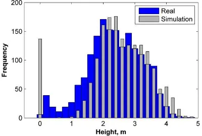
The height histograms of the simulated echoes were generally in good agreement with the real data (Figure 4), especially for birch, although there was an overestimation of mean H by 0.15–0.45 m. For the other species, the mean H was simulat-ed with reasonable accuracy, but the standard deviation (SD) was underestimated towards the highest flying altitudes. This can be due to the spatial distribution of the individual shoots, which in reality probably is more clumped at the scale of the largest footprints.
Figure 4. Real and simulated echo height histograms for 2.5– 5-m-high birch trees in the 2010_12_1 dataset.
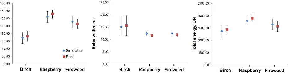
Generally, the characteristics of the radiometric WF features were well reproduced in the simulations (Figure 5). The relative interspecies order of the mean A, W and E was pre-served. The largest differences were observed for A and E of the birch in datasets 2010_12_1 and 2012_27_1, in which simulations produced 13–19% underestimations. The Npeaks was overestimated for birch in all datasets by 25–35%, which is most probably caused by the vertical gap between the crown base and the ground in the birch model (Figure 3). In reality, the gap is filled with grasses and small seedlings. In addition, there were small differences in the SD of some of the features (especially A and E) between simulated and real data. These differences varied with footprint size, which could be associated with the differences in the structure of the real and modeled plants at the footprint scale.
Figure 5. Examples of simulated and real mean WF features in the 2012_10_1 dataset. The whiskers denote standard deviation.
Absolute validation of MCRT models is difficult, because the effects of the radiative transfer model, vegetation models, and the sensor response cannot be separated from each other. Qualitative comparisons of real and simulated LiDAR data have been reported for space-borne instruments (North et al., 2010), but to our knowledge, quantitative comparisons for small-footprint airborne LiDAR have not been reported before. Our model has some uncertainties, which are related to possible errors in the vegetation modeling, exclusion of wave phenomena (interference, diffraction), improper knowledge on the scattering characteristics of the calibration targets in the hot-spot geometry, and to the simplified sensor model. In spite of the uncertainties, the results are promising and can serve as basis for attempts to calibrate and validate simulation models so that they could be used e.g. in planning of LiDAR acquisitions (Disney et al., 2010).
The computational burden is important from the practical point of view. The simulation times in the modeled vegeta-tion were 10–40 s per pulse on a standard desktop computer (Win7, 16 GB RAM, 3.33 GHz CPU). However, our algo-rithms were 'home-made' and not optimized, because the theoretical correctness was in the main focus. In addition to feasible computation times, the vegetation models should be readily available. Modeling environments already exist that could provide the input for MCRT models (e.g. Perttunen et al., 1998). Terrestrial laser scanning could be utilized as well. Independent of the method, the vegetation models should be accurate for the study area in question, or alternatively, the scattering model should be robust to the vegetation parame-ters. Improvement in the accuracy vegetation models can be expected, as interest towards computationally intensive mod-eling methods increases, and measurement data of required input parameters is accumulating.
3.2 Effects of sensor parameters on the species classifica-tion accuracy
Figure 6 shows the effect of the three investigated parameters on the overall classification accuracy of the modeled species. In general, and as expected, a higher performance was ob-tained with the less noisy 5-pulse mean features compared to individual pulse features. Classification accuracy even reached 100% with the largest simulated footprints. The three species differ quite clearly in structure, which partly explains the good classification performance. The classification accu-racies were high also in the real data for the tree species studied.
Low classification accuracies were associated with small footprints, and the accuracy saturated after approx. 0.3 mrad (0.36 m). Response to the varying pulse width was less ap-parent compared to the footprint size. Further examination revealed that, while an increase in pulse width reduces the
intraspecies variation in the WF features, it also diminishes the interspecies differences in the mean features. Sampling rate did not considerably affect the classification accuracy, although a small decrease was observed with 3–4 ns sampling in the 5-pulse data. The results indicate, that very small foot-print should be avoided if vegetation classification is aimed at. On the other hand, it appears that a 2-ns sampling rate suffices and this would reduce the storage and data transfer needs. The results can be different if more complex vegeta-tion is examined or different feature extracvegeta-tion procedures e.g. by Gaussian decomposition (Wagner et al., 2006) are implemented. Based on results here and in the Section 3.1 (different behavior of WF features with varying footprint size), we see possibilities in data that combines different footprint sizes for an enhanced classification. We propose research in this topic, not only in seedling stands but also for taller vegetation.
Figure 6. Effects of sensor parameters on the overall classifi-cation accuracy in simulated birch, raspberry and fireweed vegetation. The x axis is linear and the range from zero to the maximal values is shown.
3.3 Analyses of real data for vegetation classification
for this is probably that LiDAR underestimates the height of small trees considerably, and thus the echoes from tree crowns are still confused with low vegetation.
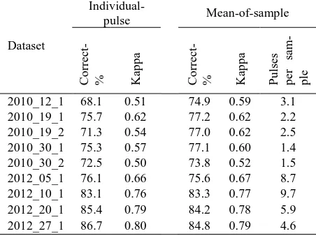
Table 2. Overall classification accuracy (%) and kappa in LDA classification of four vegetation types. Features used were the peak amplitude and total echo energy.
Dataset
The classification accuracies reported here were slightly better than obtained by Korpela et al. (2008) with similar vegetation, using DR LiDAR and high-resolution aerial images. Because we restricted to the basic pulse-vegetation phenomena, we propose further studies in the practical use of the WF data in seedling stand inventory (design of interpreta-tion techniques at the plot and stand levels). These studies could include also enhanced DEM estimation through usage of echo width features.
4 CONCLUSIONS
We presented a simulation model that integrates a sensor model and radiative transfer modeling in order to simulate LiDAR signals that are comparable to real data. Results on the model validation imply that the species-specific WF features can be simulated with the model, using literature information on the reflective properties of vegetation and simple measurements and models about the plant structure. This makes the model an excellent tool that extends empirical research e.g. when studying WF data for classification tasks. Future work could include repeating the validation procedure presented here with different kinds of vegetation, and with more accurate measurements of the calibration targets as well as the of vegetation parameters. The goal in the long time horizon is to develop simulation tools that can be utilized e.g. in planning LiDAR acquisitions, and possibly even used to produce synthetic training data. Another motivation for the study was to explore the potential of WF LiDAR data in the classification of seedling stand vegetation. The question is important, because no fully automated detection method for the silvicultural treatment need has been developed. Here, the WF signal was studied at pulse level. In the future, the analy-sis can be augmented to plot or forest stand level in order to develop practically usable inventory methods.
5 REFERENCES
Blair, J. B., Coyle, D. B., Bufton, J. L., Harding, D. J., 1994. Optimization of an airborne laser altimeter for remote sensing
of vegetation and tree canopies. In Stein, T. I. (Ed.), Proceed-ings of IGARSS’94, Pasadena, CA, 8–12 Aug, pp. 939–941.
Disney, M. I., Lewis, P., Saich, P., 2006. 3D modelling of forest canopy structure for remote sensing simulations in the optical and microwave domains. Remote Sensing of Envi-ronment, 100, pp. 114–132.
Disney, M. I., Kalogirou, V., Lewis, P., Prieto-Blanco, A., Hancock, S., Pfeifer, M., 2010. Simulating the impact of discrete-return lidar system and survey characteristics over young conifer and broadleaf forests. Remote Sensing of Envi-ronment, 114, pp. 1546–1560.
Korpela, I., Tuomola, T., Tokola, T., Dahlin, B., 2008. Ap-praisal of seedling stand vegetation with airborne imagery and discrete-return LiDAR - an exploratory analysis. Silva Fennica, 42, pp. 753–772.
Maltamo, M., Packalén, P., Kallio, E., Kangas, J., Uuttera, J., Heikkilä, J., 2011. Airborne laser scanning based stand level management inventory in Finland. In Proc. SilviLaser 2011, 16–19 Oct, Hobart, Australia, 10 p.
Morsdorf, F., Nichol, C., Malthus, T., Woodhouse, I., 2009. Assessing forest structural and physiological information content of multi-spectral LiDAR waveforms by radiative transfer modelling. Remote Sensing of Environment, 113, pp. 2152–2163.
Naesset, E., Gobakken, T., Holmgren, J., Hyyppä, H., Hyyppä, J., Maltamo, M., Nilsson, M., Olsson, H., Persson, Å., Södermalm, U., 2004. Laser scanning of forest resources: the Nordic experience. Scandinavian Journal of Forest Re-search, 19, pp. 482–499.
North, P. R. J., Rosette, J. A. B., Suarez, J. C., Los, S. O., 2010. A Monte Carlo radiative transfer model of satellite waveform LiDAR. International Journal of Remote Sensing, 31, pp. 1343–1358.
Packalén, P., Maltamo, M., 2007. The k-MSN method for the prediction of species-specific stand attributes using airborne laser scanning and aerial photographs. Remote Sensing of Environment, 109, pp. 328–341.
Perttunen, J., Sievänen R., Nikinmaa, E., 1998. LIGNUM: A Model Combining the Structure and the Functioning of Trees. Ecological Modelling, 108, pp. 189–198.
Wagner, W., Ulrich, A., Ducic, V., Melzer, T., Studnicka, N., 2006. Gaussian decomposition and calibration of a novel small-footprint full-waveform digitising airborne laser scan-ner. ISPRS Journal of Photogrammetry & Remote Sensing, 60, pp. 100–112.
Weiss, M., Baret, F., Smith, G. J., Jonckheere, I., Coppin, P., 2004. Review of methods for in situ leaf area index (LAI) determination Part II. Estimation of LAI, errors and sam-pling. Agricultural and Forest Meteorology, 121, pp. 37–53.