Economic order quantity model under fuzzy sense
when demand follows innovation diffusion process
having dynamic potential market size
K.K. Aggarwal*, Chandra K. Jaggi and
Alok Kumar
Department of Operational Research, Faculty of Mathematical Sciences, University of Delhi,
New Academic Block, Delhi 110007, India Fax: +91-11-27666672
E-mail: [email protected] E-mail: [email protected] E-mail: [email protected] *Corresponding author
Abstract: The conventional inventory models are associated with different kind of uncertainties and these uncertainties make the model unrealistic. The fuzzy set theory plays a pivotal role to address this problem. In this paper, a mathematical model has been developed for obtaining the economic order quantity (EOQ) in which the demand of the product is assumed to follow an innovation diffusion process as proposed by Fourt and Woodlock (1960). The potential market size is considered to be dynamic. To make the model more realistic an attempt has been made to solve the model in the light of fuzzy set theory under the trapezoidal membership function. The total cost formula has been derived by applying the median rule of defuzzification and the graded mean integration representation approach of defuzzification. The effectiveness of this model is illustrated with a numerical example and sensitivity analysis of the optimal solution with respect to different parameters of the system is performed.
Keywords: innovation diffusion; economic order quantity; EOQ; trapezoidal membership function; fuzzy numbers; defuzzification; function principle; median rule; graded mean integration representation method; dynamic potential market size; coefficient of innovation.
Reference to this paper should be made as follows: Aggarwal, K.K., Jaggi, C.K. and Kumar, A. (2012) ‘Economic order quantity model under fuzzy sense when demand follows innovation diffusion process having dynamic potential market size’, Int. J. Services and Operations Management, Vol. 13, No. 3, pp.361–391.
Chandra K. Jaggi is an Associate Professor in the Department of Operational Research, Faculty of Mathematical Sciences at the University of Delhi, India. He obtained his PhD, MPhil and Masters in Operational Research in the Department of Operational Research at the University of Delhi. His research interest lies on analysis of inventory system. He has more than 31 publications in Int. J. Production Economics, Journal of Operational Research Society, European Journal of Operational Research, Int. J. Systems Sciences, Canadian Journal of Pure and Applied Sciences, OPSEARCH, Investigation Operational Journal, Advanced Modelling and Optimisation, Journal of Information and Optimisation Sciences, Int. J. Mathematical Sciences, Indian Journal of Mathematics and Mathematical Sciences and Indian Journal of Management and Systems.
Alok Kumar is a Research Scholar in the Department of Operational Research, Faculty of Mathematical Sciences, University of Delhi, India. He completed his MA in Operational Research from the University of Delhi. Currently, he is pursuing his PhD in Operational Research from the Department of Operational Research, Faculty of Mathematical Sciences, University of Delhi, India. His area of research interest is inventory management and mathematical modelling.
1 Introduction
marketing or inventory management. Diffusion pattern also helps in knowing the specific characteristics of an innovative behaviour which are useful to the managers while taking important decisions in inventory management field. Therefore, innovation-diffusion theory can be useful process to assist inventory manager for planning and making strategy to determine and control the stock levels within the physical distribution function so as to balance the need for product availability and at the same time minimising the stock holding and handling costs in a situation where models developed in inventory field containing the specific characteristics of innovative behaviour of products. Because of integrated effects of globalisation, scientific advancements and other related factors, the new products are constantly entering into the market and due to its unpredictable nature the life cycles of such products are persistently reducing. Also, the potential market size is not fixed in general and it changes according to the nature of the products introduced in the market. Therefore, developing inventory models based on innovation-diffusion criterion having dynamic potential market size is the need of the hours and it also becomes essential to tackle the problems of uncertain nature of its parameters associated with it to make the inventory models realistic. In this article, an attempt has been made to develop an inventory model with demand follows innovation diffusion criterion having dynamic potential market size. The concept of fuzzy set theory has been incorporated in the model by taking some of its parameters as fuzzy numbers to make the model realistic and to improve the accuracy in decision-making. The structure of this paper has been organised as follows. Section 2 describes the literature survey to provide a theoretical background for research of the model. In Section 3, model assumptions and notations are stated which have been used later to develop the mathematical equations of this model. Section 4 describes the mathematical framework which has been developed to show the model mathematically. In Section 5, a simple solution procedure in the form of algorithm is presented to perform the numerical exercise systematically. Section 6 presents the numerical examples which have been proposed on the basis of mathematical framework developed in Section 4. To well describe the nature, behaviour and applicability of the model the separate subsections such as 6.1, 6.2 and 6.3 containing observations, discussions and managerial implications sections respectively have been well presented. Finally, the model is concluded in Section 7.
2 Literature review
unit cost under limited storage capacity. Lee and Yao (1999) discussed EOQ model in fuzzy sense for inventory without backorder. Yao and Lee (1999) developed a fuzzy inventory model with or without backorder for fuzzy order quantity with trapezoidal fuzzy number. Li et al. (2002) developed fuzzy models for single-period inventory problem. Hojati (2004) explained the probabilistic-parameter EOQ model and the fuzzy parameter EOQ model. Mandal et al. (2005) developed a multi-objective fuzzy inventory model with three constraints. Liu (2007) developed a method to find the membership function of the fuzzy profit when the demand quantity and unit cost are represented as fuzzy numbers. Benyoucef and Canbolat (2007) considered a model of fuzzy AHP-based supplier selection in e-procurement. Chen (2010) developed a model using a membership function approach to lot size re-order point inventory problems in fuzzy environments. Mahata and Goswami (2009) discussed an EOQ model with fuzzy lead time, fuzzy demand and fuzzy cost coefficients. Umap (2010) developed a fuzzy EOQ model for deteriorating items with two warehouses in which he has considered that the deteriorating rate is age specific failure rate. Tripathy et al. (2011) discussed a fuzzy EOQ model with reliability and demand-dependent unit cost. Sandeep et al. (2011) explained the application of fuzzy SMART approach for supplier selection. Chellappan and Natarajan (2011) developed a fuzzy rule-based model for the perishable collection production inventory system.
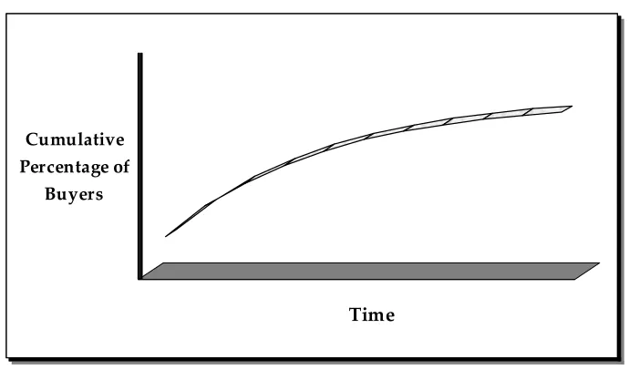
Also, the application of fuzzy set theory is highly desired when the models are developed using new product diffusion concept because new product diffusion models are based on the innovation diffusion theory and the parameters involved in it have high degree of uncertainty. The various diffusion processes have been studied in the marketing literature, which are as follows. The pure innovative model has been considered by Fourt and Woodlock (1960) whereas Fisher and Pry (1971) explain the pure imitative model. The Bass (1969) model admits both the innovative and imitative aspects of product adoption. The Bass (1969) model, introduced many years ago has been widely used in marketing by Mahajan and Muller (1979), Parker (1994), Rogers (1983, 2003, 1995) and Mahajan et al. (1990, 2000). Kalish (1985) has discussed an adoption model of a new product with price advertising and uncertainty. Mahajan and Robert (1978) have studied innovation diffusion in a dynamic potential adopter population. Sharif and Ramanathan (1982) have considered the application of dynamic potential adopter diffusion model through their study of diffusion of oral contraceptives in Thailand. The Fourt and Woodlock (1960) model explains the diffusion process in terms of number of customers who have bought the product by time ‘t’ by a modified exponential curve (Figure 1). This model captures the innovative characteristic with its coefficient ‘p’ as the coefficient of innovation. Zailani et al. (2007) considered a new product development benchmarking to enhance operation competitiveness. Rajagopal (2010) explained the case of bridging sales and service quality functions in retailing high-technology consumer products.
influenced by promotion decisions has been considered by Cheng and Sethi (1999). Sarkar et al. (2011) have developed an economic production quantity model with stochastic demand in an imperfect production system.
Figure 1 Fourt and Woodlock curve
Cumulative Percentage of
Buyers
Time
Cumulative Percentage of
Buyers
Time
Source: Lilien et al. (1999)
To develop inventory models using innovation diffusion concept under fuzzy environment will be advantageous for a number of reasons. Therefore, in this paper, an inventory model is developed where demand of the product is assumed to follow an innovation diffusion process as considered by Fourt and Woodlock (1960) model under a strict assumption that the potential market size is dynamic. To make the model more realistic, an attempt has been made to solve the model in the light of fuzzy set theory under the trapezoidal membership function. A numerical example and a comprehensive sensitivity analysis have been provided to illustrate the results of the proposed model. The results obtained using two methods of defuzzification such as median rule of defuzzification and graded mean integration representation method of defuzzification have been compared to know the practical utility of the model. The calculated results provide significant impetus while taking inventory decisions for new products.
2.1 Purely innovative diffusion process
Pure innovative models assume that the diffusion takes place due to innovation or external influence. Fourt and Woodlock (1960) model is the earliest pure innovative model. The demand model considered in this paper is purely innovative in nature. In this section, we very briefly discuss Fourt and Woodlock model, which will be used later on to conceptualise the demand model to find the optimal EOQ policy. The model is mostly used in the form
1
(1 )t
t
where
Qt sales at time ‘t’ which is a fraction of the potential sales Q total potential sales as fraction of all buyers
r rate of penetration of untapped potential t time period.
The model assumes that the level of adoption capability Qt can be expressed as a function of time t and generate an exponential declining curve of new-adopter sales over time. The values for the parameter Q and r, can be estimated on the basis of available historical data points in such a way that the resulting curve fits the data well.
On the basis of this curve, future adoption can be forecasted.
3 Assumptions and notations
The model emphasises a case which is concerned with the diffusion models of new product acceptance having objective to represent the level of spread of an innovation among a given set of prospective buyers. Here, the mathematical model developed is based on the framework of innovation diffusion criterion which is influenced by the Fourt and Woodlock (1960) model. The demand model considered here is time dependent and having the functional form as n t( )=λ( )t = p N t[ ( )−N t( )] which is based on Fourt and Woodlock (1960). The constant parameter ‘p’ mentioned in the demand function represented as a coefficient of innovation and interpreted as reflecting the extent of a consumer’s intrinsic propensity to purchase the product. The coefficient of innovation may also be stated as the likelihood that somebody who is not yet using the product will start using it because of mass media coverage or other external factors. For t≥ 0, N(t) is the cumulative number of adopters of a product by time ‘t’ in a large target population. The potential market size of total number of adopters is not constant but dynamic in nature which is time dependent and has been denoted here as N t( ). Assume that the time interval ‘T’ is given and we are to plan an inventory policy for a certain commodity during time interval ‘T’ by using the demand rate λ(t) as explained above with its certain assumptions which are as follows. The replenishment rate is infinite implies that the replenishments are instantaneous. Lead time is zero and shortages are not allowed. There is only one product bought per new adopter. The innovation’s sales are confined to a single geographical area and it is assumed that there is no seasonality in sales of the new product. It is considered that the impacts of marketing strategies by the innovator are adequately captured by the model’s parameters.
In addition, the following notations will be used in developing the proposed model: A ordering cost per order
C unit cost
IC inventory carrying cost
T length of the replenishment cycle
Q number of items received at the beginning of the period p coefficient of innovation
K(T) the total cost of the system per unit time I(t) on hand inventory at any time t
n(t) = λ(t) = S(t) the number of adoptions at time t, i.e., demand at time t N0 initial potential market size.
4 Mathematical model
The basic demand model used in this paper is based on the following assumptions: 1 adoptions take place due to innovation-diffusion process and it is influenced by the
innovation-effect (mass-media) only
2 the innovation effect is constant throughout the cycle time 3 the potential market size is time dependent (dynamic).
The demand model used in this paper is based on the hypothesis that there exists potential market whose size is time dependent (dynamic). With the passage of time prospective buyers adopt the product. Using (1) and the demand assumptions, the mathematical form of rate adoption at any time ‘t’ can be given as:
( )
( ) ( )
1 ( )
f t
t p t p
F t
ϕ = = =
− (2)
where
ϕ(t) is the hazard rate that gives the conditional probability of a purchase in a small time interval (t, t + Δt), if the purchase has not occurred till time ‘t’
f(t) is the likelihood of purchase at time ‘t’
0
( ) ( )
t
F t =
∫
f t dt is the cumulative likelihood of purchasing the product at time ‘t’. Equation (2) can be rewritten as[
]
( )( ) 1 ( ) ; where ( ) ( )
N t
f t p F t F t
N t
= − = (3)
( ) accept a new product independently of the decisions of others in a dynamic potential market size which varies with time.
It is true with the fact that the potential market size in case of new product diffusion does not remain constant with time. It varies with time. It may decrease or increase as time passes. The potential market size of a product may decrease for that product itself if its substitute product enters into the market and it may increase linearly or exponentially or follows any other distribution for a number of reasons such as bringing different kind of promotional efforts like advertising, discounting, etc. and by imparting external influences among people of the society. Here, we have considered a case when potential market size increases exponentially.
Now, when potential market size increases exponentially
0
to be as fuzzy numbers.
0
Therefore, ( )λ t =n t( )= p N e⎣⎡ gt−N t( ) ,⎤⎦ g>0 (6) The demand usage λ(t) which is a function of time plays pivotal role to shrink the
inventory size over a period of time. If in the time interval (t, t + dt) the inventory size is dipping at the rate λ(t)dt, then the total reduction in the inventory size during the time interval dt can be given by –dI(t) = λ(t)dt. Thus, differential equation describing the
Using the equations (6) and (7) we get
0
The solution of the differential equation (8) is:
(
)
0
Using the equations (9) and (12) we get
(
)
The total cost of inventory system per unit time consists of the following elements: Ordering cost per unit time (OC) A
T
= (15)
Material cost per unit time (MC) QC T
Cost of carrying inventory per unit time (IHC) ( )
Let the inventory carrying charge ‘I’ in fuzzy sense be represented by ‘ ’I that is I is supposed to be as fuzzy number.
Therefore, equation (19) can be written as follows
(
)
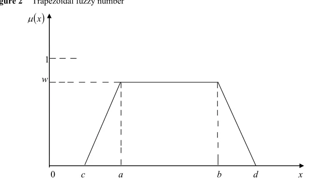
fuzzy numbers have been used by making use of trapezoidal membership function.Now the trapezoidal membership function μA( )x for the fuzzy numbers is described as follows:
Figure 2 Trapezoidal fuzzy number
( )
xμ
1
w
0 c a b d x
Let p N, 0 and I be the fuzzy numbers with the trapezoidal membership function as defined in equation (22) such as
(
1, 2, 3, 4)
p = p p p p (23)
(
)
0 01, 02, 03, 04
N = N N N N (24)
(
1, 2, 3, 4)
I= I I I I (25)
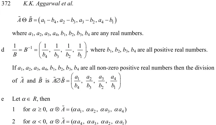
Now, in order to make simpler the calculation of trapezoidal fuzzy number, here, we use the Chen’s (1985) function principle to calculate the fuzzy total cost per unit time of our proposed model under the following fuzzy arithmetical operations. We apply this principle for the operation of addition, subtraction, multiplication and division of fuzzy numbers.
Suppose A=( , , , )a1 a2 a3 a4 and B=( , , , )b1 b2 b3 b4 are two trapezoidal fuzzy numbers. Then
a The addition of A and B is
(
1 1, 2 2, 3 3, 4 4)
A⊕ =B a +b a +b a +b a +b
where a1, a2, a3, a4, b1, b2, b3, b4 are any real numbers.
b The multiplication of A and B is A⊗ =B ( , , , )c1 c2 c3 c4 where
λ = (a1b1, a1b4, a4b1, a4b4), λ1 = (a2b2, a2b3, a3b2, a3b3) c1 = min λ, c2 = min λ1, c3 = max λ1, c4 = max λ.
If a1, a2, a3, a4, b1, b2, b3, b4 are all non-zero positive real numbers, then
(
1 1, 2 2, 3 3, 4 4)
A⊗ =B a b a b a b a b
(
1 4, 2 3, 3 2, 4 1)
Therefore, using the function principle method the membership function of K T( ) can be defined as
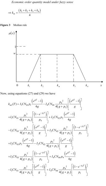
The total cost per unit time containing fuzzy numbers is calculated using defuzzification method. Here, we have used two kinds of defuzzification method, one is median rule and the other is graded mean integration representation method to calculate total cost per unit time of the system.
Case 1 Defuzzification of total cost per unit time using median rule
(
1 2 3 4)
Now, using equations (27) and (29) we have
(
)
Now, again by applying median rule of defuzzification as discussed in equations (28) and (29) and also explained through Figure 3, the lot size Q as obtained in equation (12) represented in fuzzy sense after defuzzification as Qm1 for Case 1 has been described as follows:
For optimum total cost, the necessary criterion is
(
)
satisfies the condition2
dT > Since the above cost equation (34) is highly non-linear, the problem has been solved numerically for given parameter values. The solution gives the optimum value T* of the replenishment cycle time T. Once T* is known the value of optimum order quantity Qm1 and the optimum cost km1(T*) can easily be obtained from the equations (32) and (30), respectively. The numerical solution for the given base value has been obtained by using software packages LINGO and Excel-Solver.
Case 2 Defuzzification of total cost per unit time using graded mean integration representation method
The graded mean integration representation method based on the integral value of graded mean h-level of fuzzy number was proposed by Chen and Hsieh (1999) has been described as follows.
and represented in Figure 4. Therefore, the graded mean integration representation of A denoted as K A( ) is
Hence, to defuzzify the total cost variable using graded mean integration representation method under trapezoidal membership function the km has been defined as follows:
(
1 2 2 2 3 4)
( )
(
)
For optimum total cost, the necessary criterion is
(
)
(
)
(
)
(
)
satisfies the condition2
5 Solution procedure
Here, the aim of our model is to determine the optimum value of T which minimises the total cost per unit time such as km1(T) and km2(T) for median rule of defuzzification and graded mean integration representation method of defuzzification respectively for fixed values of other parameters associated with it. This optimum value of T will also help in getting the optimum lot size which eventually assists in mentioning the reorder point. The detailed step-wise solution procedure to calculate the optimum cycle length, optimum total cost and the optimum lot size has been summarised in the following algorithm. Step 1 Input all parameter values such as different cost parameters, coefficient of
innovation, potential market size, etc. with three parameters on which sensitivity analysis is to be performed separately such as inventory carrying charge, coefficient of innovation and potential market size are to be taken in the form of fuzzy numbers for both the cases median rule as well as graded mean integration representation method.
Step 2 Compute all possible values of ‘T’ using equation (34) and equation (41) for Case 1 and Case 2, respectively.
Step 3 Select the appropriate value of ‘T’ separately using equation (35) and equation (42) for Case 1 and Case 2, respectively. Here, the value of T is to be considered as optimal cycle length denoted as T* which will minimise km1(T) and km2(T) and will satisfy the conditions
2 graded mean integration representation method respectively.
Step 4 Compute km1(T*) and km2(T*) for the optimum value T* obtained in Step 3 using equation (30) and equation (38) for Case 1 and Case 2, respectively and hence calculate the corresponding value of Qm1(T*) and Qm2(T*) using equation (32) and equation (39) for median rule and graded mean integration representation method respectively.
The above steps are used for all replenishment schedules using appropriate parameter values. In order to obtain the values of ‘T’, we need to solve the equation (30) for Case 1 and equation (38) for Case 2 using LINGO and EXCEL-Solver software packages.
6 Numerical examples
The behaviour and application of the proposed model have been shown here by the following numerical analysis. Consider a hypothetical example in an inventory system with the following parameters in an appropriate units as follows:
0
$1,100/order, $300/unit, 0.20, (10, 000, 15, 000, 20, 000, 25, 000) (0.10, 0.15, 0.20, 0.25) and (0.005, 0.006, 0.007, 0.008)
A C g N
( )
( )
0.37, 43, 631, 46 (using median rule)
0.38, 44, 027, 46.97 (using graded mean integration representation method) cost and the optimum order quantity of the inventory model has been shown numerically in the following numerical tables using the above stated solution procedure. Also, to prove the validity of the model numerically and to get the appropriate parameter values, the references have been considered as Chanda and Kumar (2011, 2012), Chandrasekaran and Tellis (2007), Sultan et al. (1990), Talukdar et al. (2002), Van den Bulte and Stremersch (2004), and Aggarwal et al. (2011).
Case 1 Numerical tables based on median rule
Table 1 Sensitivity analysis on coefficient of innovation ‘ ’p
p T* km1(T*) Qm1(T*)
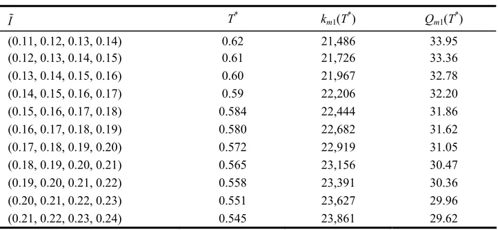
Table 2 Sensitivity analysis on inventory carrying charge ‘ ’I
Table 3 Sensitivity analysis on initial potential market size ‘N0’
0
N T* km1(T
*
) Qm1(T *
)
(10,000, 11,000, 1,2000, 13,000) 0.715 14,603 23.44
(11,000, 12,000, 13,000, 14,000) 0.691 15,675 24.62
(12,000, 13,000, 14,000, 15,000) 0.660 16,743 25.28
(13,000, 14,000, 15,000, 16,000) 0.643 17,807 26.22
(14,000, 15,000, 16,000, 17,000) 0.625 18,868 27.03
(15,000, 16,000, 17,000, 18,000) 0.602 19,925 27.74
(16,000, 17,000, 18,000, 19,000) 0.593 20,980 29.01
(17,000, 18,000, 19,000, 20,000) 0.574 22,031 29.36
(18,000, 19,000, 20,000, 21,000) 0.565 23,081 30.62
(19,000, 20,000, 21,000, 22,000) 0.553 24,128 31.25
(20,000, 21,000, 22,000, 23,000) 0.546 25,173 32.11
Notes: For p=(0.001, 0.002, 0.003, 0.004) I=(0.10, 0.15, 0.20, 0.25)
Case 2 Numerical tables based on graded mean integration representation method
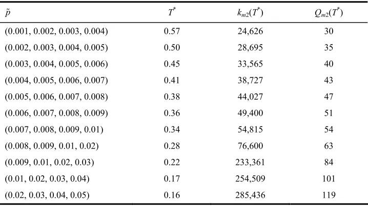
Table 4 Sensitivity analysis on coefficient of innovation ‘ ’p
p T* km2(T*) Qm2(T*)
(0.001, 0.002, 0.003, 0.004) 0.57 24,626 30
(0.002, 0.003, 0.004, 0.005) 0.50 28,695 35
(0.003, 0.004, 0.005, 0.006) 0.45 33,565 40
(0.004, 0.005, 0.006, 0.007) 0.41 38,727 43
(0.005, 0.006, 0.007, 0.008) 0.38 44,027 47
(0.006, 0.007, 0.008, 0.009) 0.36 49,400 51
(0.007, 0.008, 0.009, 0.01) 0.34 54,815 54
(0.008, 0.009, 0.01, 0.02) 0.28 76,600 63
(0.009, 0.01, 0.02, 0.03) 0.22 233,361 84
(0.01, 0.02, 0.03, 0.04) 0.17 254,509 101
(0.02, 0.03, 0.04, 0.05) 0.16 285,436 119
Table 5 Sensitivity analysis on inventory carrying charge ‘ ’I
I T* km2(T
*
) Qm2(T *
)
(0.11, 0.12, 0.13, 0.14) 0.63 21,836 33.01
(0.12, 0.13, 0.14, 0.15) 0.62 22,158 32.55
(0.13, 0.14, 0.15, 0.16) 0.61 22,479 32.11
(0.14, 0.15, 0.16, 0.17) 0.605 22,799 31.72
(0.15, 0.16, 0.17, 0.18) 0.601 23,119 31.50
(0.16, 0.17, 0.18, 0.19) 0.593 23,438 31.05
(0.17, 0.18, 0.19, 0.20) 0.585 23,756 30.61
(0.18, 0.19, 0.20, 0.21) 0.573 24,073 29.95
(0.19, 0.20, 0.21, 0.22) 0.570 24,390 29.78
(0.20, 0.21, 0.22, 0.23) 0.564 24,706 29.45
(0.21, 0.22, 0.23, 0.24) 0.557 25,022 29.06
Notes: For p=(0.001, 0.002, 0.003, 0.004) N0=(10,000, 15,000, 20,000, 25,000)
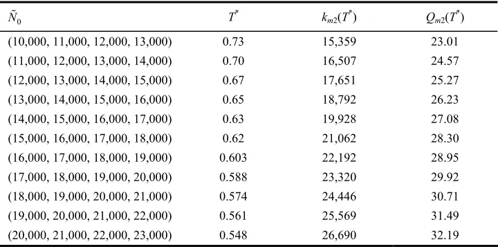
Table 6 Sensitivity analysis on initial potential market size ‘N0’
0
N T* km2(T*) Qm2(T*)
(10,000, 11,000, 12,000, 13,000) 0.73 15,359 23.01
(11,000, 12,000, 13,000, 14,000) 0.70 16,507 24.57
(12,000, 13,000, 14,000, 15,000) 0.67 17,651 25.27
(13,000, 14,000, 15,000, 16,000) 0.65 18,792 26.23
(14,000, 15,000, 16,000, 17,000) 0.63 19,928 27.08
(15,000, 16,000, 17,000, 18,000) 0.62 21,062 28.30
(16,000, 17,000, 18,000, 19,000) 0.603 22,192 28.95
(17,000, 18,000, 19,000, 20,000) 0.588 23,320 29.92
(18,000, 19,000, 20,000, 21,000) 0.574 24,446 30.71
(19,000, 20,000, 21,000, 22,000) 0.561 25,569 31.49
(20,000, 21,000, 22,000, 23,000) 0.548 26,690 32.19
Notes: For p=(0.001, 0.002, 0.003, 0.004) I=(0.10, 0.15, 0.20, 0.25)
6.1 Observations
in Table 1 and Table 4. This is consistent with the reality as more investment on promotion will increase the diffusion of a product in the market resulting in shrinkage of the optimal reorder cycle time as a result optimal cost is increased. b As depicted in Table 2 and Table 5, it has been observed in both the cases that as the
average value of inventory carrying charge increases keeping other parameters constant then both the optimal cycle length T* and the optimal order quantity Qmi(T*) decreases while the optimal total cost kmi(T*) increases. This is true with the fact that as inventory carrying charge increases, it compels the inventory manager to keep the inventory for reduced time period which leads to shrinkage of ordered quantity and in that process optimum total cost is increased due to increment in the ordering cost because of addition in the number of orders.
c On the basis of results obtained in Table 3 and Table 6, it has been observed in both the cases that as the average value of potential market size increases keeping other parameters constant then the optimal cycle length T* decreases while both the optimal order quantity Qmi(T*) and the optimal total cost kmi(T*) increases. This is explained as the growth of potential market size may increase the number of adopters which will force the inventory manager to keep more inventories for short time period to keep itself from fading out from the market as a result optimal cost is increased.
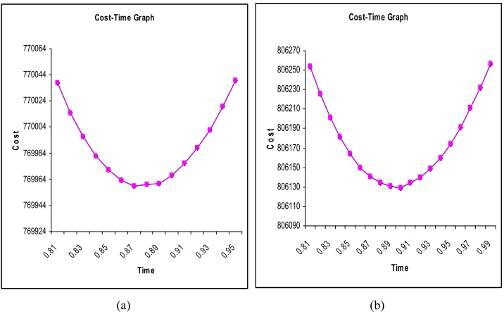
d If we compare the results obtained in the above six tables for both the cases separately, it can be clearly shown that the median rule of defuzzification is more suitable for this model than the graded mean integration representation method of defuzzification. Here, the suitability of defuzzification method has been judged on the basis of comparative results obtained for optimum cycle time, optimum total cost and the optimal order quantity for both the cases separately.
Figure 5 Cost-time graphs showing convexity of the cost functions for (a) Case 1 and (b) Case 2 (see online version for colours)
6.2 Discussion
The parameters involved in the inventory models are generally not fixed and cannot be predicted with certainty. These parameters fluctuate in their domain from the actual values. Hence, assuming constant parameters which are vague in nature and performing sensitivity analysis on a fixed parameter will make the inventory models unrealistic and will not give the desired results. This model is based on the new product diffusion concept and the parameters such as coefficient of innovation, potential market size, etc. associated with it are of uncertain nature which makes the model unrealistic. Therefore, to make the model realistic and to improve the accuracy in the desired results, here, three parameters namely coefficient of innovation, inventory carrying charge and the potential market size have been taken as fuzzy numbers and the sensitivity analysis of the model has been performed on these three parameters. The behaviour and sensitive nature of these parameters have been well explained in the observation section. On the basis of results obtained in the above six numerical tables, the comparative study of the two methods of defuzzification used in this model clearly shows that the median rule of defuzzification is more suitable for this model than the graded mean integration representation method of defuzzification. Therefore, this model will help the decision-makers while taking optimum decisions if the nature of the problems are matched with such model having specific characteristics as discussed above and moreover this model will facilitate in reducing the level of uncertainty in case of those parameters which are of uncertain nature and are calculated by converting them in fuzzy numbers.
6.3 Managerial implications
7 Conclusions
Acknowledgements
The authors are thankful to the anonymous reviewers and the editor for their constructive comments and suggestions. This paper has been revised in light of their suggestions and comments.
References
Aggarwal, K.K., Jaggi, C.K. and Kumar, A. (2011) ‘Economic order quantity model with innovation diffusion criterion having dynamic potential market size’, International Journal of Applied Decision Sciences, Vol. 4, No. 3, pp.280–303.
Bass, F.M. (1969) ‘A new-product growth model for consumer durables’, Management Science, Vol. 15, No. 5, pp.215–227.
Benyoucef, M. and Canbolat, M. (2007) ‘Fuzzy AHP-based supplier selection in e-procurement’, International Journal of Services and Operations Management, Vol. 3, No. 2, pp.172–192. Chanda, U. and Kumar, A. (2011) ‘Economic order quantity model with demand influenced by
dynamic innovation effect’, International Journal of Operational Research, Vol. 11, No. 2, pp.193–215.
Chanda, U. and Kumar, A. (2012) ‘Economic order quantity model on inflationary conditions with demand influenced by innovation diffusion criterion’, International Journal of Procurement Management, Vol. 5, No. 2, pp.160–177.
Chandrasekaran, D. and Tellis, G.J. (2007) ‘A critical review of marketing research on diffusion of new products’, Review of Marketing Research, Vol. 3, pp.39–80.
Chellappan, E.C. and Natarajan, M. (2011) ‘Fuzzy rule based model for the perishable collection-production-inventory system’, International Journal of Management Science and Engineering Management, Vol. 6, No. 3, pp.183–190.
Chen, S.H. (1985) ‘Operation on fuzzy numbers with function principle’, Tamkang Journal of Management Sciences, Vol. 6, No. 1, pp.13–26.
Chen, S.H. and Hsieh, C.H. (1999) ‘Graded mean integration representation of generalized fuzzy number’, Journal of Chinese Fuzzy Systems, Vol. 5, No. 2, pp.1–7.
Chen, S.P. (2010) ‘A membership function approach to lot size re-order point inventory problems in fuzzy environments’, International Journal of Production Research, Vol. 49, No. 13, pp.3855–3871.
Chen, S-H., Wang, C-C. and Arthur, R. (1996) ‘Backorder fuzzy inventory model under function principle’, Information Sciences, Vol. 95, Nos. 1–2, pp.71–79.
Cheng, F. and Sethi, S. (1999) ‘A periodic review inventory model with demand influenced by promotion decisions’, Management Science, Vol. 45, No. 11, pp.1510–1523.
Chern, M.S., Teng, J.T. and Yang, H.L. (2001) ‘Inventory lot-size policies for the bass diffusion demand models of new durable products’, Journal of the Chinese Institute of Engineers, Vol. 24, No. 2, pp.237–244.
Fisher, J.C. and Pry, R.H. (1971) ‘A simple substitution model of technological change’, Technological Forecasting and Social Change, Vol. 3, No. 2, pp.75–88.
Fourt, L.A. and Woodlock, J.W. (1960) ‘Early prediction of market success for new grocery products’, The Journal of Marketing, Vol. 25, No. 2, pp.31–38.
Hojati, M. (2004) ‘Bridging the gap between probabilistic and fuzzy-parameter EOQ models’, International Journal of Production Economics, Vol. 91, No. 3, pp.215–221.
Kacprzyk, J. and Staniewski, P. (1982) ‘Long-term inventory policy making through fuzzy decision making models’, Fuzzy Sets and Systems, Vol. 8, No. 2, pp.117–132.
Lee, H.M. and Yao, J.S. (1999) ‘Economic order quantity in fuzzy sense for inventory without back order model’, Fuzzy Sets and Systems, Vol. 105, No. 1, pp.13–31.
Li, L., Kabadi, S.N. and Nair, K.P.K. (2002) ‘Fuzzy models for single-period inventory problem’, Fuzzy Sets and Systems, Vol. 132, No. 3, pp.273–289.
Lilien, G.P., Kotler, P. and Moorthy, K.S. (1992) Marketing Models, Prentice Hall, New Jersey. Liu, S.T. (2007) ‘Fuzzy profit measures for a fuzzy economic order quantity model’, Applied
Mathematical Modeling, Vol. 32, No. 10, pp.2076–2086.
Mahajan, V. and Muller, E. (1979) ‘Innovation diffusion and new-product growth models in marketing’, The Journal of Marketing, Fall, Vol. 43, No. 4, pp.55–68.
Mahajan, V. and Robert, P. (1978) ‘Innovation diffusion in a dynamic potential adopter population’, Management Science, Vol. 24, No. 15, pp.1589–1597.
Mahajan, V., Muller, E. and Bass, F.M. (1990) ‘New product diffusion models in marketing: a review and directions for research’, The Journal of Marketing, Vol. 54, No. 1, pp.1–26. Mahajan, V., Muller, E. and Wind, Y. (2000) New-Product Diffusion Models, Kluwer Academic
Publisher, Boston, MA.
Mahata, G.C. and Goswami, A. (2009) ‘An EOQ model with fuzzy lead time, fuzzy demand and fuzzy cost coefficients’, International Journal of Engineering and Applied Sciences, Vol. 5, No. 5, pp.295–302.
Mandal, N.K., Roy, T.K. and Maiti, M. (2005) ‘Multi-objective inventory model with three constraints: a geometric programming approach’, Fuzzy Sets and Systems, Vol. 150, No. 1, pp.87–106.
Park, K.S. (1987) ‘Fuzzy-set theoretic interpretation of economic order quantity’, IEEE Transactions on Systems, Man and Cybernets SMC, Vol. 17, No. 6, pp.1082–1084.
Parker, P.M. (1994) ‘Aggregate diffusion forecasting models in marketing: a critical review’, International Journal of Forecasting, Vol. 10, No. 2, pp.353–380.
Petrovic, D., Petrovic, R. and Vujosevic, M. (1996) ‘Fuzzy models for the newsboy problem’, International Journal of Production Economics, Vol. 45, No. 1, pp.435–441.
Rajagopal (2010) ‘Bridging sales and service quality functions in retailing high-technology consumer products’, International Journal of Services and Operations Management, Vol. 7, No. 2, pp.177–199.
Rogers, E.M. (1962) Diffusion of Innovations, The Free Press, New York.
Rogers, E.M. (1983, 2003) Diffusion of Innovations, 3rd ed., Free Press, New York. Rogers, E.M. (1995) Diffusion of Innovations, 4th ed., Free Press, New York.
Roy, T.K. and Maiti, M. (1997) ‘A fuzzy EOQ model with demand-dependent unit cost under limited storage capacity’, European Journal of Operational Research, Vol. 99, No. 2, pp.425–432.
Sandeep, M., Kumanan, S. and Vinodh, S. (2011) ‘Application of fuzzy SMART approach for supplier selection’, International Journal of Services and Operations Management, Vol. 9, No. 3, pp.365–388.
Sarkar, B., Sana, S.S. and Chaudhuri, K. (2011) ‘An economic production quantity model with stochastic demand in an imperfect production system’, International Journal of Services and Operations Management, Vol. 9, No. 3, pp.259–283.
Sharif, M.N. and Ramanathan, K. (1982) ‘Polynomial innovation diffusion models’, Technological Forecasting and Social Change, Vol. 21, No. 4, pp.301–323.
Sommer, G. (1981) ‘Fuzzy inventory scheduling’, in Lasker, G. (Ed.): Applied Systems and Cybernetics, Vol. 6, pp.3052–3060, Pergamon Press, New York.
Sultan, F., Farley, J.U. and Lehmann, D.R. (1990) ‘A meta-analysis of applications diffusion models’, Journal Of Marketing Research, Vol. 27, No. 1, pp.70–77.
Tripathy, P.K., Tripathy, P. and Pattnaik, M. (2011) ‘A fuzzy EOQ model with reliability and demand-dependent unit cost’, Int. J. Contemp. Math. Sciences, Vol. 6, No. 30, pp.1467–1482. Umap, H.P. (2010) ‘Fuzzy EOQ model for deteriorating items with two warehouses’, Journal of
Statistics and Mathematics, Vol. 1, No. 2, pp.1–6.
Van den Bulte, C. and Stremersch, S. (2004) ‘Social contagion and income heterogeneity in new product diffusion: a meta-analytic test’, Marketing Science, Vol. 23, No. 4, pp.530–544. Yao, J.S. and Lee, H.M. (1999) ‘Fuzzy inventory with or without backorder for fuzzy order
quantity with trapezoid fuzzy number’, Fuzzy Sets and Systems, Vol. 105, No. 3, pp.311–337. Zadeh, L.A. (1965) ‘Fuzzy sets’, Information and Control, Vol. 8, No. 3, pp.338–353.