Economic order quantity model with innovation
diffusion criterion having dynamic potential market
size
K.K. Aggarwal*, Chandra K. Jaggi and
Alok Kumar
Department of Operational Research, Faculty of Mathematical Sciences, New Academic Block, University of Delhi,
Delhi 110007, India
Abstract: Introduction of a new product in the market forces the inventory managers to consider the effects of marketing policies especially for innovation effects at the earlier stage of the product life cycle to make the economic order quantity (EOQ) model more realistic. Traditional EOQ models generally do not consider the effect of marketing parameters. In this paper, a time dependent innovation driven demand model has been introduced in the basic EOQ model to calculate the different optimal policies. This model assumes that potential market size is dynamic over time. The proposed model acknowledges relationship between the innovation coefficient and the optimal policies. The effectiveness of this model is illustrated with a numerical example and sensitivity analysis of the optimal solution with respect to different parameters of the system is performed.
Keywords: economic order quantity; EOQ; innovation driven demand; dynamic potential adopters; diffusion theory.
Reference to this paper should be made as follows: Aggarwal, K.K., Jaggi, C.K and Kumar, A. (2011) ‘Economic order quantity model with innovation diffusion criterion having dynamic potential market size’, Int. J. Applied Decision Sciences, Vol. 4, No. 3, pp.280–303.
Biographical notes: K.K. Aggarwal is an Assistant Professor in the Department of Operational Research at University of Delhi, India. He obtained his MSc in Operational Research and PhD in Inventory Management from University of Delhi. His research interests and teaching include inventory modelling, financial engineering and network analysis. He has published more than 15 research papers in many scholarly journals.
Journal of Pure and Applied Sciences, OPSEARCH, Investigation Operational Journal, Advanced Modelling and Optimisation, Journal of Information and Optimisation Sciences, Int. J. Mathematical Sciences, Indian Journal of Mathematics and Mathematical Sciences and Indian Journal of Management and Systems.
Alok Kumar is a Research Scholar in the Department of Operational Research, Faculty of Mathematical Sciences, University of Delhi, India. He received his MA in Operational Research from University of Delhi. Currently, he is pursuing his PhD in Operational Research from the Department of Operational Research, Faculty of Mathematical Sciences, University of Delhi, India. His area of research interest include inventory management and mathematical modelling.
1 Introduction
The economic ordering policies often depend on demand information and demand is mainly influenced by different marketing strategies. Therefore, the appropriate modelling of demand is of great importance. Particularly, it is more significant for the new products, because demands of such products are highly dynamic in nature and have less predictable growth behaviour. In inventory system, normally demand of product is considered to be constant, time dependent, stock dependent or probabilistic in nature. Unfortunately, inventory modelling generally do not take into account the demand pattern of new products. Changing needs of the society, technological breakthroughs the impact of globalisation forces manufacturers to introduce new products in the market. When new products are introduced in the market, their inventory management becomes significant. The economic order quantity (EOQ) models have been explored to a great extent, in particular with their interaction to different functional areas of business management like production and finance. Though some models are there that used the Bass diffusion demand model to formulate the optimal EOQ model (Chern et al., 2001) but not much of work has been reported on the interaction of EOQ with marketing strategies. The integration of EOQ policies with marketing policies is one of the key factors of successful business operation. Therefore, the coordination between marketing disciplines and inventory management is yet to be explored fully.
The proposed model includes the integration of EOQ with marketing disciplines in which demand follows innovation diffusion process with dynamic market potential size. Diffusion modelling of new product adoption has become an active area of marketing research with more emphasis on inventory management since the pioneering work of Bass (1969). This model is concerned with representing the dynamic nature of the adoption of a new product. Since diffusion models are normative in nature and models of this type include managerial decision variables in order to study their effect on the diffusion process, therefore, here, role of inventory manager becomes indispensable while managing the inventory and hence the importance of mathematical modelling in inventory for such kind of situation is highly desired.
penetration of a market by a new product. One of the most widely held theories of communication in marketing is diffusion theory. Diffusion theory is actually a theory of communication regarding how information is disseminated within a social system over time. An innovation is an idea, object or a practice that is perceived as novel by the members of the social system. Individuals who constitute the market may differ by the manner in which the information about the innovation reaches to them and the manner in which they respond to such received information. Diffusion is defined as the process by which an innovation is communicated through certain channels over time among members of a social system (Rogers, 1983, 2003).
diffusion model that can be used to forecast the diffusion of an innovation at early stages of the diffusion curve. Niu (2006) developed a piecewise-diffusion model of new-product demands. Puumalainen et al. (2007) developed a model which proposes a set of uncertainty sources of telecommunications industry that have notable effect on the diffusion of innovations in the field. Chandrasekaran and Tellis (2007) have studied a critical review of marketing research on diffusion of new products. Stremersch et al. (2010) described the importance of time which accelerates early growth of new products. Shinohara and Okuda (2010) proposed a dynamic innovation diffusion modelling. Peres et al. (2010) have studied a critical review of innovation diffusion and new product growth models.
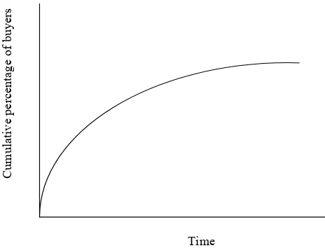
Figure 1 Increments of new-buyer penetration
Time
Source: Fourt and Woodlock (1960, pp.33–34)
The Fourt and Woodlock model explains the diffusion process in terms of number of customers who have bought the product by time t by a modified exponential curve (Figure 1). The discrete form of the model can be given as:
1
Q total potential sales as fraction of all buyers r rate of penetration of untapped potential t time period.
The model assumes that the level of adoption capability Qt can be expressed as a function
The Fourt and Woodlock model and many other researchers in the marketing disciplines usually assume that the potential market size remains constant over time, but in reality, it is not always possible. Different promotional activities, increase in purchasing power due to increase in income, increase in population and several other factors lead to increase in potential market size over time. Therefore, it becomes important to include the potential market as dynamic instead of constant as far as research regarding innovation diffusion is concerned. Sharif and Ramanathan (1982) have considered the application of dynamic potential adopter diffusion model through their study of diffusion of oral contraceptives in Thailand.
In this paper, an inventory model is developed where it is assumed that demand of the product follows innovation diffusion behaviour as considered by Fourt and Woodlock model and potential market size is dynamic. A comprehensive sensitivity analysis is performed to highlight the impact of diffusion of innovation on the economic ordering policies. The calculated results provide significant impetus while taking inventory decisions for new products. This article is divided into model development, special cases and observations and concludes with a discussion on the application.
2 Mathematical models
2.1 Assumptions and notations
Inventory model has been developed under the following assumptions: 1 the replenishment rate is instantaneous
2 lead time is zero
3 shortages are not allowed
4 demand rate is known and is governed by innovation process
5 the size of the potential market of total number of adopters is dynamic in nature 6 the coefficient of innovation is constant in nature
7 the innovation’s sales are confined to a single geographical area. Notations used in the modelling framework are as follows:
A Ordering cost.
C Unit cost.
p(t) Innovation effect at time t. Here, p(t) = p we assume that the innovation factor that influences consumer adoption decision will remain constant during the entire product life cycle.
I Inventory carrying charge. IC Inventory carrying cost.
T Length of the replenishment cycle.
K(T) The total cost of the system per unit time. I(t) On hand inventory at any time t.
n(t) = λ(t) = S(t) The number of adoptions at time t, i.e., demand at time t. 0
N Initial potential market size.
N(t) Cumulative number of adopters at time t.
The basic demand model used in this paper is based on the following assumptions: 1 Adoptions take place due to innovation-diffusion process and it is influenced by the
innovation-effect (mass-media) only.
2 The innovation effect is constant throughout the cycle time.
3 The potential market size is time dependent (dynamic). In this way, two form of time dependent potential market size, i.e., linear and exponential have been considered by taking two different cases.
The demand model used in this paper is based on the hypothesis that there exists potential market whose size is time dependent (dynamic). With the passage of time prospective buyers adopt the product. Using (1) and the demand assumptions, the mathematical form of rate adoption at any time t can be given as:
The physical interpretation of the above model is the probability that a potential adopter will purchase a product at time t given that no purchase has occurred till time t.
where
ϕ(t) is the hazard rate that gives the conditional probability of a purchase in a small time interval (t, t + ∆t), if the purchase has not occurred till time Equation (2) can be rewritten as:
[
]
1 when potential market size increases linearly taking, N t( )=N0(1+gt) g>0
2 when potential market size increases exponentially taking, N t( )=N e0 gt g>0
Case 1 when potential market size increases linearly
Taking, N t( )=N0(1+gt) Therefore,
0
( )t n t( ) p N (1 gt) N t( )
λ = = ⎡⎣ + − ⎤⎦ (4)
The demand usage λ(t) which is a function of time plays pivotal role to shrink the inventory size over a period of time. If in the time interval (t, t + dt) the inventory size is dipping at the rate λ(t)dt, then the total reduction in the inventory size during the time interval dt can be given by –dI(t) = λ(t)dt. Thus, differential equation describing the
Using equations (4) and (5) we get
0
The solution of the differential equation (6) is:
(
)
Since replenishment is instantaneous and shortages are not allowed. Therefore,
Using the equations (7) and (8) we get
Now,
The total cost per unit time, K1(T) comprises of the following elements
a ordering cost per unit time
1
(OC) A
T
= (10)
b inventory holding cost per unit time
(
)
c material cost per unit time
(
1)
1 0 0 1(
pT 1)
Using the equations (10), (11) and (12) we get
Therefore,
dT > Since the above cost equation (13) is highly
non-linear, the problem has been solved numerically for given parameter values. The solution gives the optimum value T* of the replenishment cycle time T. Once T* is known the value of optimum order quantity Q* and the optimum cost K1(T*) can easily be
obtained from the equations (8) and (13) respectively. The numerical solution for the given base value has obtained by using software packages LINGO and Excel-Solver. Case 2 When potential market size increases exponentially
Taking, N t( )=N e0 gt
0
Using the equations (16) and (17) we get
0
The solution of the differential equation (18) is: 2
Since replenishment is instantaneous and shortages are not allowed. Therefore,
Using the equations (19) and (20) we get
(
)
2(
) (
)
The total cost per unit time, K2(T) comprises of the following elements
(
2)
A OC
T
= (22)
b inventory holding cost per unit time
(
)
(
)
c material cost per unit time
(
2)
2 0(
)
0 2(
) (
)
Using the equations (22), (23) and (24) we get
Now, for K2(T) to be convex
dT > Since the above cost equation (25) is highly
non-linear, the problem has been solved numerically for given parameter values. The solution gives the optimum value T* of the replenishment cycle time T. Once T* is known the value of optimum order quantity Q* and the optimum cost K2(T*) can easily be
obtained from the equations (20) and (25) respectively. The numerical solution for the given base value has obtained by using software packages LINGO and Excel-Solver.
2.2 Special case
When N t( ) becomes constant over a period of time say N then demand rate, i.e.,
For optimum total cost, the necessary criterion is
dT > Since the above cost equation is highly non-linear,
the problem has been solved numerically for given parameter values. The solution gives the optimum value T* of the replenishment cycle time T. Once T* is known the value of optimum order quantity Q* and the optimum cost K(T*) can easily be obtained by following the same procedure as obtained in the above two cases. The numerical solution for the given base value has obtained by using software packages LINGO and Excel-Solver.
3 Solution procedures
The solution procedure has been summarised in the following algorithm
Step 1 Input all parameter values such as unit cost, coefficient of innovation, potential market size, ordering cost etc. for each case separately.
Step 2 Compute all possible values of T separately for the equations (14), (26) and (29) as the case may be.
Step 3 Select the appropriate value of T for each case by using the equations (13), (25) and (28) and by satisfying the above stated condition such as
2
The above steps are used for all replenishment cycles using appropriate parameter values. In order to obtain the appropriate values of T we need to follow the above procedure with the help of LINGO and EXCEL-Solver software packages.
4 Numerical examples
A numerical example is presented in the following to illustrate the effectiveness of the proposed model. A hypothetical example has the following parameter values in appropriate units.
$1, 000/order, $1, 050/unit, 30%
Using the solution procedure described above, the optimal values of cycle length, order quantity and total cost under different cases have been presented in Tables 1 to 5 for different parameter values. Also, to prove the validity of the model numerically and to get the appropriate parameter values, the references have been considered as Sharif and Ramanathan (1981), Chandrasekaran and Tellis (2007), Sultan et al. (1990), Talukdar et al. (2002) and Van den Bulte and Stremersch (2004).
• The mean value of the coefficient of innovation for a new product usually lies between 0.0007 and 0.03 (Sultan et al., 1990; Talukdar et al., 2002; Van den Bulte and Stremersch, 2004).
• The mean value of the coefficient of innovation for a new product is usually 0.001 for developed countries and 0.0003 for developing countries (Talukdar et al., 2002). Case 1 When potential market size increases linearly
For this case, Sharif and Ramanathan (1981) considered the Coleman model and explained by taking the case study of credit card banking in the USA. Here, Sharif and Ramanathan (1981) regard this model as Model-1(b) and took the following parameter values.
0 1459.77, 0.1292
N = α = =g
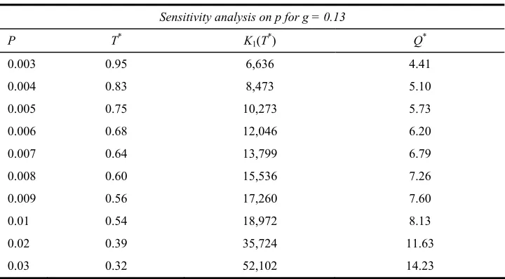
Table 1 shows the changes in the values of T, Q and K1(T) for variations in the values of
coefficient of innovation for fixed value of g, whereas, Table 2 describes the changes with respect to g for fixed value of coefficient of innovation.
Table 1 Changes in optimal values due to p
Sensitivity analysis on p for g = 0.13
P T* K1(T*) Q*
0.003 0.95 6,636 4.41
0.004 0.83 8,473 5.10
0.005 0.75 10,273 5.73
0.006 0.68 12,046 6.20
0.007 0.64 13,799 6.79
0.008 0.60 15,536 7.26
0.009 0.56 17,260 7.60
0.01 0.54 18,972 8.13
0.02 0.39 35,724 11.63
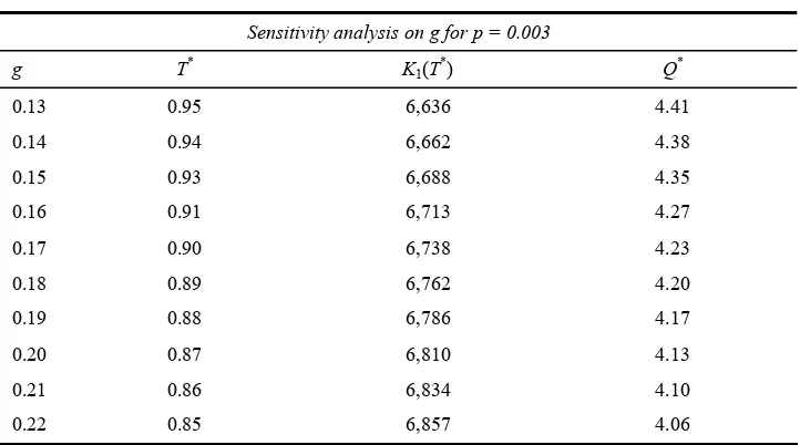
Table 2 Changes in optimal values due to g
Sensitivity analysis on g for p = 0.003
g T* K1(T*) Q*
0.13 0.95 6,636 4.41
0.14 0.94 6,662 4.38
0.15 0.93 6,688 4.35
0.16 0.91 6,713 4.27
0.17 0.90 6,738 4.23
0.18 0.89 6,762 4.20
0.19 0.88 6,786 4.17
0.20 0.87 6,810 4.13
0.21 0.86 6,834 4.10
0.22 0.85 6,857 4.06
Case 2 When potential market size increases exponentially
In this case, Sharif and Ramanathan (1981) took the following parameter values. 2
0 1928.55, 2.5863 10
N = α = =g ×
Table 3 shows the changes in the values of T, Q and K2 (T) for variations in the values of
coefficient of innovation for fixed value of g, whereas, Table 4 describes the changes with respect to g for fixed value of coefficient of innovation.
Table 3 Changes in optimal values due to p
Sensitivity analysis on p for g = 0.13
P T* K2(T*) Q*
0.003 0.99 8,065 5.77
0.004 0.86 10,391 6.67
0.005 0.77 12,680 7.46
0.006 0.71 14,942 8.25
0.007 0.66 17,184 8.94
0.008 0.61 19,410 9.44
0.009 0.58 21,623 10.09
0.01 0.55 23,825 10.63
0.02 0.40 45,461 15.42
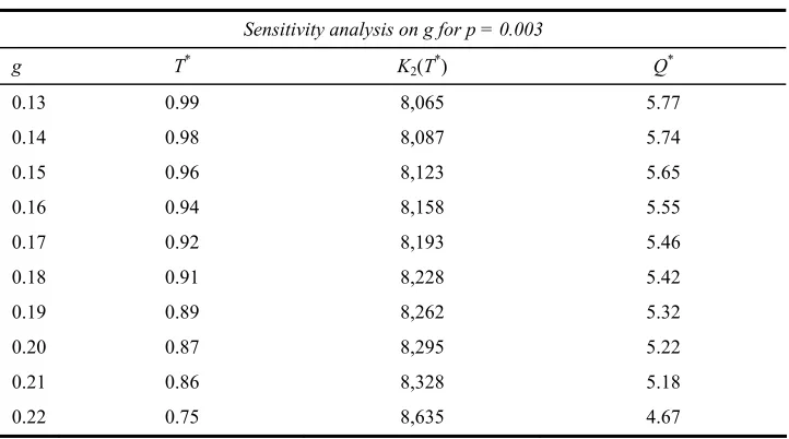
Table 4 Changes in optimal values due to g
Sensitivity analysis on g for p = 0.003
g T* K2(T*) Q*
0.13 0.99 8,065 5.77
0.14 0.98 8,087 5.74
0.15 0.96 8,123 5.65
0.16 0.94 8,158 5.55
0.17 0.92 8,193 5.46
0.18 0.91 8,228 5.42
0.19 0.89 8,262 5.32
0.20 0.87 8,295 5.22
0.21 0.86 8,328 5.18
0.22 0.75 8,635 4.67
4.1 Special case
In this case, Sharif and Ramanathan (1981) considered the following parameter values.
0 2441.78, 0
N = α = =g
Table 5 shows the changes in the values of T, Q and K(T) for variations in the values of coefficient of innovation.
Table 5 Changes in optimal values due to p
Sensitivity analysis on p
p T* K(T*) Q*
0.003 0.91 5,047 6.65
0.004 0.81 6,425 7.89
0.005 0.70 7,818 8.52
0.006 0.62 9,194 9.06
Following graphs show the behaviour of optimal total cost and optimal cycle length with the changes in the coefficient of innovation for different cases.
Case 1 When potential market size increases linearly
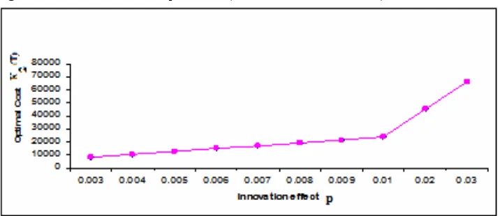
Figure 2 Innovation effects vs. optimal cost (see online version for colours)
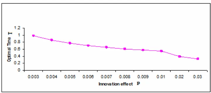
Figure 3 Innovation effect vs. optimal time (see online version for colours)
Case 2 When potential market size increases exponentially
Figure 4 presents the impact of coefficient of innovation on optimal total cost and Figure 5 shows the impact on optimal cycle length.
Figure 5 Innovation effect vs. optimal time (see online version for colours)
4.2 Special case
Figure 6 presents the impact of coefficient of innovation on optimal total cost and Figure 7 shows the impact on optimal cycle length.
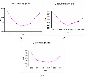
It can be seen that it is very difficult to prove the convexity of total cost curves in equations (13), (25) and (28) analytically. The convexity of total cost curves has been checked graphically for all the cases. Figures 8(a) to 8(c) illustrate the convexity of total cost curves for different cases.
Figure 7 Innovation effect vs. optimal time (see online version for colours)
Figure 8 Cost graphs showing convexity of the cost functions for (a) case 1, (b) case 2 and (c) special case (see online version for colours)
(a) (b)
5 Observations
We study the effect of changes in the system parameters on the optimal values of total cost K(T*), the optimal cycle length T* and the optimal order quantity Q(T*). The results obtained in the numerical exercise are very encouraging and are consistent with the reality. From the results of numerical exercise and the graphical representation (Figures 2, 3, 4, 5, 6 and 7) it has been observed that:
a As the values of p increase keeping other parameters constant, the value of T* start decreasing, the optimal order quantity Q(T*) increases slightly while the optimal cost K(T*) increases significantly as depicted in Tables 1, 3 and 5. This is consistent with the reality as more investment on promotion will increase the diffusion of a product in the market resulting in shrinkage of the optimal reorder cycle time as a result optimal cost is increased.
b As the values of g increases keeping other parameters constant the value of T* and the optimal order quantity Q(T*) decreases marginally while there is slight increase in the optimal cost K(T*) as depicted in Tables 2 and 4. This kind of phenomenon usually occurs in the real life situation as increment in g makes the potential adopter dynamic which forces the inventory manager to keep the inventories according to the changing pattern of the cycle time to get the total cost optimal.
6 Managerial implications
organisation for scheduling and managing the inventories when new products are introduced in the dynamic potential market.
7 Conclusions
To manage and control inventory of a new product becomes a challengeable task for almost every organisation because it requires a huge amount of investment of capital to purchase inventory. Therefore, it becomes indispensable to develop a mathematical model to get rid of these problems, as mathematical models are ideal tools to control and manage the inventories of a new product in most economical way. In this paper, a time dependent innovation driven demand model with dynamic potential market size has been introduced in the basic EOQ model to calculate the different optimal policies. The proposed model acknowledged relationship between the innovation coefficient and the optimal policies in a dynamic market environment of two kinds. The results are very encouraging and the findings are consistent with the idea that optimal EOQ policies are highly sensitive towards the dynamics of innovation coefficient in a dynamic environment and it is imperative to identify a trend. A numerical example followed by sensitivity analysis on model parameters has been provided to verify the results obtained in the real life situation. A simple solution procedure in the form of algorithm is presented to determine the optimal cycle time and optimal order quantity of the cost function. A special case has also been formulated which excludes the dynamic nature of the potential market size.
A few limitations in our approach that suggests areas for future research, are as follows. As the proposed EOQ model uses the extension of pure innovative demand model, hence it ignores imitation coefficient (Bass, 1969) which is an important factor in consumer adoption decision. The existence and the uniqueness of the different cost functions have been shown numerically because of its highly non-linear nature. Thus research on some alternative approach to get the optimal analytical solution of the problem is important. In further research, we would like to extend the proposed model for multiple generation situations, shortages, partial lost-sales, quantity discount etc.
Acknowledgements
The authors would like to thank the anonymous reviewers and the editor for their constructive comments and suggestions.
References
Agarwal, R. and Bayus, B.L. (2002) ‘The market evolution and sales takeoff of product innovations’, Management Science, Vol. 48, No. 8, pp.1024–1041.
Alfares, H.K., Khursheed, S.M. and Noman, S.M. (2005) ‘Integrating quality and maintenance decisions in a production-inventory model for deteriorating items’, International Journal of Production Research, Vol. 43, No. 5, pp.899–911.
Bass, F.M. (1969) ‘A new product growth model for consumer durables’, Management Sci., Vol. 15, pp.215–227.
Blackman, W.A., Jr., Seligman, E.J. and Solgliero, G.C. (1973) ‘An innovation index based upon factor analysis’, Technological Forecasting and Social Change, Vol. 4, pp.301–316.
Chanda, U. and Bardhan, A.K. (2008) ‘Modelling innovation and imitation sales of multiple technological generation products’, Journal of High Technology Management Research, Vol. 18, No. 2, pp.173–190, DOI: 10.1016/j.hitech. 2007.12.004.
Chandrasekaran, D. and Tellis, G.J. (2007) ‘A critical review of marketing research on diffusion of new products’, Review of Marketing Research, pp.39–80.
Cheng, F. and Sethi, S. (1999) ‘A periodic review inventory model with demand. influenced by promotion decisions’, Management Science, Vol. 45, No. 11, pp.1510–1523.
Chern, M.S., Teng, J.T. and Yang, H.L. (2001) ‘Inventory lot-size policies for the bass diffusion demand models of new durable products’, Journal of the Chinese Institute of Engineers, Vol. 24, No. 2, pp.237–244.
Danaher, P.J., Hardie, B.G.S. and Putsis, W.P., Jr. (2001) ‘Marketing-mix variables and the diffusion of successive generations of a technological innovation’, Journal of Marketing Research, Vol. 38, No. 4, pp.501–514.
Dodson, J.A., Jr. and Muller, E. (1978) ‘Models of new product diffusion through advertising and word-of-mouth’, Journal of Marketing,Vol. 24, No. 15, pp.1–26.
Everdingen, Y.M.V., Aghina, W.B. and Fok, D. (2005) ‘Forecasting cross-population innovation diffusion: a Bayesian approach’, International Journal of Research in Marketing, Vol. 22, pp.293–308.
Fisher, J.C. and Pry, R.H. (1971) ‘A simple substitution model of technological change’, Technological Forecasting and Social Change, Vol. 3, pp.75–88.
Fourt, L.A. and Woodlock, J.W. (1960) ‘Early prediction of market success for new grocery products’, Journal of Marketing, Vol. 25, pp.31–38.
Furukawa, R. and Kato, H. (2002) ‘A conceptual model for adoption and diffusion process of a new product’, Review of Marketing Science, Vol. 1, No. 1, pp.1–28.
Golder, P.N. and Tellis, G.J. (1998) ‘Beyond diffusion: an explanatory approach to modeling the growth of durables’, Journal of Forecasting, Vol. 17, pp.259–280.
Hamblin, R.L., Jacobsen, R.B. and Miller, J.L. (1973) A Mathematical Theory of Social Change, John Wiley & Sons, Inc., New York, NY.
Henard, D.H. and Szymanski, D.M. (2001) ‘Why some new products are more successful than others’, Journal of Marketing Research, Vol. 38, pp.362–375.
Jaber, M.Y., Bonney, M. and Moualek, I. (2009) ‘An economic order quantity model for an imperfect production process with entropy cost’, International Journal of Production Economics, Vol. 118, pp.26–33.
Kalish, S. (1985) ‘A new product adoption model with price advertising and uncertainty’, Management Science, Vol. 31, No. 12, pp.1569–1585.
Kurawarwala, A.A. and Matsuo, H. (1996) ‘Forecasting and inventory management of short life-cycle products’, Operations Research, Vol. 44, No. 1, pp.131–150.
Lilien, G.L., Kotler, P. and Moorthy, K.S. (1999) Marketing Models, Prentice-Hall of India Private Limited, New Delhi.
Linton, J.D. (2002) ‘Forecasting the market diffusion of disruptive and discontinuous innovation’, IEEE Transactions on Engineering Management, Vol. 49, No. 4, pp.365–374.
Mahajan, V. and Muller, E. (1979) ‘Innovation diffusion and new-product growth models in marketing’, Journal of Marketing Fall, Vol. 43, pp.55–68.
Mahajan, V. and Robert, A.P. (1978) ‘Innovation diffusion in a dynamic potential adopter population’, Management Science, Vol. 24, No. 15.
Mahajan, V., Muller, E. and Bass, F.M. (1990a) ‘New product diffusion models in marketing: areview and directions for research’, The Journal of Marketing, Vol. 54, No. 1, pp.1–26. Mahajan, V., Muller, E. and Srivastava, R.K. (1990b) ‘Determination of adopter, categories using
innovation diffusion models’, Journal of Marketing, Vol. 27, No. 1, pp.37–50.
Mahajan, V., Muller, E. and Bass, F.M. (1995) ‘Diffusion of new products empirical generalizations and managerial uses’, Marketing Science, Vol. 14, No. 3, pp.G79–G88.
Mahajan, V., Muller, E. and Wind, Y. (2000) New-Product Diffusion Models, Kluwer Academic Publisher, Boston, MA.
Masao, N. (1973) ‘Advertising and promotion effects on consumers response to new products’, Journal of Marketing Research, Vol. 10, pp.242–249.
Niu, S.C. (2006) ‘A piecewise-diffusion models of new-product demands’, Operations Research, Vol. 54, No. 4, pp.678–695.
Pae, J.H. and Lehmann, D.R. (2003) ‘Multigeneration innovation diffusion: the impact of intergeneration time’, Journal of the Academy of Marketing Science, Vol. 31, No. 1, pp.36–45. Parker, P.M. (1994) ‘Aggregate diffusion forecasting models in marketing: a critical review’,
International Journal of Forecasting, Vol. 10, pp.353–380.
Peres, R., Muller, E. and Mahajan, V. (2010) ‘Innovation diffusion and new product growth models: a critical review and research directions’, International Journal of Research in Marketing, Vol. 27, pp.91–106.
Puumalainen, K., Sundqvist, S. and Huiskonen, J. (2007) ‘Managing uncertainty in forecasting the diffusion of telecommunications innovations’, Journal of Scientific and Industrial Research, Vol. 66, pp.299–304.
Robert, G.B. (1973) ‘A model for measuring the influence of promotion and consumer demand’, Journal of Marketing Research, Vol. 10, No. 4, pp.380–389.
Roberts, J.H. (2000) ‘Developing new rules for new markets’, Journal of the Academy of Marketing Science, Vol. 28, No. 1, pp.31–44.
Roberts, J.H. and Urban, G. (1988) ‘Modeling multivariate utility, risk, and belief dynamics for new consumer durable brand choice’, Management Science, Vol. 34, No. 2, pp.167–185. Rogers, E.M. (1962) Diffusion of Innovations, The Free Press, New York.
Rogers, E.M. (1983, 2003) Diffusion of Innovations, 3rd ed., The Free Press, New York. Rogers, E.M. (1995) Diffusion of Innovations, 4th ed., The Free Press, New York.
Sharif, M.N. and Ramanathan, K. (1981) ‘Binomial innovation models with dynamic potential adopter population’, Technological Forecasting and Social Change, Vol. 20, pp.63–87. Sharif, M.N. and Ramanathan, K. (1982) ‘Polynomial innovation diffusion models’, Technological
Forecasting and Social Change, Vol. 21, pp.301–323.
Shinohara, K. and Okuda, H. (2010) ‘Dynamic innovation diffusion modeling’, Comput. Econ, Vol. 35, pp.51–62.
Stremersch, S., Muller, E. and Peres, R. (2010) ‘Does new product growth accelerate across technology generations’, Journal of Marketing, Vol. 21, No. 2, pp.103–120.
Sultan, F., Farley, J.U. and Lehmann, D.R. (1990) ‘A meta-analysis of diffusion models’, Vol. 27, No. 1, pp.70–77.
Talukdar, D., Sudhir, K. and Ainslie, A. (2002) ‘Investigating new product diffusion across products and countries’, Marketing Science, Vol. 21, No. 1, pp.97–114.
Van den Bulte, C. (2000) ‘New product diffusion acceleration: measurement and analysis’, Marketing Science, Vol. 19, No. 4, pp.366–380.
Van den Bulte, C. and Lilien, G.L. (2001) ‘Medical innovation revisited: contagion versus marketing effort’, The American Journal of Sociology, Vol. 106, No. 5, pp.1409–1435. Van den Bulte, C. and Stremersch, S. (2004) ‘Social Contagion and income heterogeneity in new