Full Terms & Conditions of access and use can be found at
http://www.tandfonline.com/action/journalInformation?journalCode=ubes20
Download by: [Universitas Maritim Raja Ali Haji] Date: 12 January 2016, At: 23:41
Journal of Business & Economic Statistics
ISSN: 0735-0015 (Print) 1537-2707 (Online) Journal homepage: http://www.tandfonline.com/loi/ubes20
Optimal Power for Testing Potential Cointegrating
Vectors With Known Parameters for
Nonstationarity
Graham Elliott, Michael Jansson & Elena Pesavento
To cite this article: Graham Elliott, Michael Jansson & Elena Pesavento (2005) Optimal Power for Testing Potential Cointegrating Vectors With Known Parameters for Nonstationarity, Journal of Business & Economic Statistics, 23:1, 34-48, DOI: 10.1198/073500104000000307
To link to this article: http://dx.doi.org/10.1198/073500104000000307
View supplementary material
Published online: 01 Jan 2012.
Submit your article to this journal
Article views: 43
Optimal Power for Testing Potential
Cointegrating Vectors With Known
Parameters for Nonstationarity
Graham E
LLIOTTUniversity of California, San Diego 9500 Gilman Drive, La Jolla, CA 92093 (gelliott@weber.ucsd.edu)
Michael J
ANSSONUniversity of California, Berkeley, Berkeley, CA 94720
Elena P
ESAVENTOEmory University Atlanta, GA 30322
Theory often specifies a particular cointegrating vector among integrated variables, and testing for a unit root in the known cointegrating vector is often required. Although it is common to simply use a univariate test for a unit root for this test, it is known that this does not take into account all available information. We show here that in such testing situations, a family of tests with optimality properties exists. We use this to characterize the extent of the loss in power from using popular methods, as well as to derive a test that works well in practice. We also characterize the extent of the losses of not imposing the cointegrating vector in the testing procedure. We apply various tests to the hypothesis positing that price forecasts from the Livingston data survey are cointegrated with prices, and find that although most tests fail to reject the presence of a unit root in forecast errors, the tests presented here strongly reject this (implausible) hypothesis.
KEY WORDS: Cointegration; Optimal test; Unit root.
1. INTRODUCTION
This article examines tests for cointegration when the re-searcher knows the cointegrating vector a priori and when the “X” variables in the cointegrating regression are known to be integrated of order one [I(1)]. In particular, we characterize a family of optimal tests for the null hypothesis of no cointe-gration when there is one cointegrating vector. This enables us to examine the loss in power from suboptimal methods (e.g., univariate unit root tests on the cointegrating vector) and also losses that arise from testing cointegration with estimated coin-tegrating vectors.
There are a number of practical reasons for our interest in this family of tests. First, in many applications a potential coin-tegrating vector is specified by economic theory (see Zivot 2000 for a list of examples), and researchers are confident or willing to assume that variables are I(1). The test of interest then becomes testing whether the implied cointegrating vector has a unit root (which would falsify the theory). The empiri-cal strategy commonly followed is to simply construct the po-tential cointegrating vector and use a univariate test for a unit root. However, this method avoids using useful information in the original multivariate model that could lead to more pow-erful tests (see Zivot 2000). Although tests are available that do exploit this extra information in the problem (e.g., those in Horvath and Watson 1995; Johansen 1988, 1995; Kremers, Ericsson, and Dolado 1992; Zivot 2000), these tests do not use this information optimally. The class of tests suggested herein, identical apart from the treatment of deterministic terms to those of Elliott and Jansson (2003) for testing for unit roots with stationary covariates, do have optimality properties.
Second, the optimal family that we derive allows the power bound of such tests to be derived. This is interesting in the
sense that it gives an objective for examining the loss of power in estimating rather than specifying the cointegrating vector. A quantitative understanding of this loss and how it varies with nuisance parameters of the model is important for understand-ing differences in empirical results. If one researcher specifies the parameters of the cointegrating vector and rejects while an-other estimates the vector and fails to reject, then we are more certain that this is likely due to loss of power when there are large losses in power from estimating the cointegrating vector. If the power losses were small, then we would probably con-clude that the imposed parameters are in error. By deriving the results analytically, we are able to say what types of models (or, more concretely, what values for a certain nuisance para-meter) are likely to be related to large or small power losses in estimating the cointegrating vector. For many values of the nuisance parameter (which is consistently estimable and is pro-duced as a byproduct of the test proposed herein) the differ-ences in power is large.
Section 2 presents our model and relates it to error-correction models (ECMs). Section 3 considers tests for cointegration when the cointegrating vector is known. We discuss a number of approaches that have been used in the literature and present the methods of Elliott and Jansson (2003) in the context of this problem. Section 4 presents numerical results to show the asymptotic and small sample performances of the Elliott and Jansson (2003) test relative to others in the literature. Section 5 describes an empirical application relating to the cointegration of forecasts and their outcomes.
© 2005 American Statistical Association Journal of Business & Economic Statistics January 2005, Vol. 23, No. 1 DOI 10.1198/073500104000000307
34
2. THE MODEL AND ASSUMPTIONS
We consider the case where a researcher observes an (m+1)-dimensional vector time serieszt=(yt,x′t)′generated the lag operatorL,and the following assumptions hold:
Assumption 1. max−k≤t≤0(uy,t,u′x,t)′ = Op(1), where
· is the Euclidean norm.
Assumption 2. |A(r)| =0 has roots outside the unit circle.
Assumption 3. Et−1(εt)=0 (a.s.), Et−1(εtε′t)= (a.s.), and suptEεt2+δ<∞for some δ >0,where is positive definite and Et−1(·) refers to the expectation conditional on
{εt−1,εt−2, . . .}.
We are interested in the problem of testing
H0:ρ=1 versus H1:−1< ρ <1.
Under the maintained hypothesis,xtis vector-integrated process whose elements are not mutually cointegrated. There is no coin-tegration betweenyt andxt under the null, whereasyt andxt are cointegrated under the alternative because yt −γ′xt = µy +τyt+uy,t mean reverts to its deterministic component when −1< ρ <1.We assume that the researcher knows the value ofγ, the parameter that characterizes the potentially coin-tegrating relation betweenytandxt.This assumption is plausi-ble in many empirical applications, including the one discussed in Section 5. We entertain various assumptions onµy,µx,τy, andτx.
Assumptions 1–3 are fairly standard and are the same as (A1)–(A3) of Elliott and Jansson (2003). Assumption 1 ensures that the initial values are asymptotically negligible, Assump-tion 2 is a staAssump-tionarity condiAssump-tion, and AssumpAssump-tion 3 implies that
{εt} satisfies a functional central limit theorem (e.g., Phillips and Solo 1992).
There are a number of different vector autoregressive (VAR)-type representations of the model in (1)–(3). Ignoring deterministic terms for the sake of exposition, we now present three such representations, each of which sheds light on the properties of our model and the precise restrictions of the for-mulation of the foregoing problem. The restrictions are pre-cisely those embodied in the idea thatxt is known to beI(1) under both the null and alternative hypotheses.
A general ECM representation for the data is
˜
A(L)[Im+1(1−L)−αβ′L]zt=εt, (4) where β=(1,−γ′)′. Comparing this with the (1) form, we note that the two representations are equivalent when α =
((ρ−1),0)′, whereαis(m+1)×1 and also
These are precisely the restrictions on the full system that impose the assumed knowledge over the system that we are exploiting as well as the correct normalization on the root of interest when testing for a unit root in the known cointegrating vector.
First, becauseA˜(L)is a rotation ofA(L), the roots of each lag polynomial are equivalent, and hence Assumption 2 rules out the possibility of other unit roots in the system. Second, the normalization of the first element ofαto(1−ρ)merely ensures that the root that we are testing is scaled correctly under the alternative.
The important restriction is setting elements 2 throughm+1 ofαto0, which is the typical assumption in the triangular form. This restriction is precisely the restriction that thext’s are con-strained to be I(1)under the null and alternative—this is the known information that the testing procedures developed here are intended to exploit. We assume thatxt isI(1)in the sense that the weak limit ofT−1/2x[T
·] is a Brownian motion under
the null and local alternatives of the formρ=1+T−1c,where
cis a fixed constant.
To see this, we show that if zt is generated by (4) and As-sumptions 1–3 hold, thenxtisI(1)under local alternatives only ifα=(ρ−1)(1,0′)′.Now suppose thatzt is generated by (4) and ⇒ denotes weak convergence, it is easy to show that
T−1/2[T·] under local alternatives if and only if αx=0, as claimed. It follows from the foregoing discussion that ifαxwere nonzero in (5), then under the null hypothesis we would have thatxtis
I(1)whereas under the alternative hypothesis, we would sud-denly have a small but asymptotically nonnegligible persistent component in xt. This would be an artificial difference be-tween the null and alternative models that is unlikely to map into any real life problem.
A second form of the model is the ECM representation of the model,
where we have partitionedA(L)after the first row and column. From this formulation, we are able to see that xt is weakly exogenous forγ if and only ifA(1)is block upper triangular when partitioned after the first row and column (i.e., elements 2 throughm+1 of the first column ofA(1)are equal to 0). Thus the “directional” restriction that we place onαand the restric-tion on the ECM implicit in the triangular representarestric-tion are distinct from the assumption of weak exogeneity. They become equivalent only when there is no serial correlation [i.e., when A(L)=Im+1]. We do not impose weak exogeneity in general.
Finally, our model can be written as
A(L) can be represented as a VAR model of the form examined by Elliott and Jansson (2003). Apart from deterministic terms, the testing problem studied here is therefore isomorphic to the unit root testing problem studied by Elliott and Jansson (2003). In the next section we use the results of that work to construct powerful tests for the testing problem under consideration here.
3. TESTING POTENTIAL COINTEGRATING VECTORS WITH KNOWN PARAMETERS
FOR NONSTATIONARITY
3.1 Existing Methods
There are a number of tests derived for the null hypothe-sis considered in this article. An initial approach (for the PPP hypothesis see, e.g., Cheung and Lai 2000; for income con-vergence see Greasley and Oxley 1997 and, in a multivariate setting, Bernard and Durlauf 1995) was to realize that withγ
known, one could simply undertake a univariate test for a unit root inyt−γ′xt.Any univariate test for a unit root inyt−γ′xt is indeed a feasible and consistent test; however, this amounts to examining (1) ignoring information in the remainingm equa-tions in the model. As is well understood in the stationary con-text, correlations between the error terms in such a system can be exploited to improve estimation properties and the power of hypothesis tests. For the testing problem under consideration here, we have that under both the null and alternative hypothe-ses, the remaining m equations can be fully exploited to im-prove the power of the unit root test. Specifically, there is extra exploitable information available in the “known” stationarity ofxt.[That such stationary variables can be used to improve power is evident from the results of Hansen (1995) and Elliott and Jansson (2003).] The key correlation that describes the availability of power gains is the long-run (“zero frequency”) correlation between uy,t and ux,t. In the case where this correlation is zero, an optimal univariate unit root test is op-timal for this problem. Outside of this special case many tests have better power properties. There is still a small sample is-sue: Univariate tests require fewer estimated parameters. This is analyzed in small-sample simulations in Section 4.4.
For a testing problem analogous to ours, Zivot (2000) used the covariate augmented Dickey–Fuller test of Hansen (1995) usingxtas a covariate. Hansen’s (1995) approach extends the approach of Dickey and Fuller (1979) to testing for a unit root
by exploiting the information in stationary covariates. These tests deliver large improvements in power over univariate unit root tests, but they do not make optimal use of all available information. The analysis of Zivot (2000) proceeds under the assumption thatxt is weakly exogenous for the cointegrating parametersγ under the alternative. In addition, Zivot (2000, p. 415) assumed (as do we) thatxtisI(1). As discussed in the previous section, these two assumptions are different in gen-eral even though they are equivalent in the leading special case when there is no serial correlation [i.e., whenA(L)=Im+1]. The theoretical analysis of Zivot (2000) therefore proceeds un-der assumptions that are identical to ours in the absence of serial correlation and strictly stronger than ours in the presence of se-rial correlation. Similarly, all local asymptotic power curves of Zivot (2000) are computed under assumptions that are strictly stronger than ours in the presence of serial correlation.
One could also use a trace test to test for the number of cointegrating vectors when the cointegrating vectors are pre-specified. Horvath and Watson (1995) computed the asymptotic distribution of the test under the null and the local alternatives. The trace test does exploit the correlation between the errors to increase power, but does not do so optimally for the model that we consider. We show numerically that the power of the Horvath and Watson (1995) test is always below the power of the Elliott and Jansson (2003) test when it is known that the covariates areI(1). All of the tests that we consider are able to distinguish alternatives other than the one on which we fo-cus in this article; however, for none of these alternatives (say,
αx is nonzero) are optimality results available for any of the tests. This lack of any optimality result means that we have no theoretical prediction as to which test is the best test for those models. This implication is brought out in simulation results showing that the rankings between the statistics change for var-ious models when the assumption thatxtisI(1)under the alter-native is relaxed.
3.2 Optimal Tests
The development of optimality theory for the testing prob-lem considered here is complicated by the nonexistence of a uniformly most powerful (UMP) test. Nonexistence of a UMP test is most easily seen in the special case whereγ=0andxtis strictly exogenous. In that case our testing problem is simply that of testing ifythas a unit root, and it follows from the results of Elliott, Rothenberg, and Stock (1996) that no UMP-invariant (to the deterministic terms) test exists. By implication, a like-lihood ratio test statistic constructed in the standard way will not give tests that are asymptotically optimal. That the more general model is more complicated than this special case will not override this lack of optimality on the part of the likelihood ratio test. Elliott and Jansson (2003) therefore returned to first principles to construct tests that will enjoy optimality proper-ties. Apart from the test suggested here, none of the tests dis-cussed in the previous section are in the family of optimal tests discussed here except in special cases (i.e., particular values for the nuisance parameters). In this section we describe the deriva-tion of the test of Elliott and Jansson (2003), the funcderiva-tional form of which is presented in the next section.
Given values for the parameters of the model other thanρ [i.e.,A(L),µy,µx,τy,andτx] and a distributional assumption
of the formεt∼iidF(·)[for some known cdfF(·)], it follows from the Neyman–Pearson lemma that a UMP test of
H0:ρ=1 versus Hρ¯:ρ= ¯ρ
exists and can be constructed as the likelihood ratio test be-tween the simple hypothesesH0andHρ¯.Even in this special
case, the statistical curvature of the model implies that the func-tional form of the optimal test statistic depends on the simple alternativeHρ¯ chosen. To address this problem, one could
fol-low Cox and Hinkley (1974, sec. 4.6) and construct a test that maximizes power for a given size against a weighted average of possible alternatives. (The existence of such a test follows from the Neyman–Pearson lemma.) Such a test, with the test statistic denoted byψ({zt},G|A(L), µy,µx, τy,τx,F), would then max-imize (among all tests with the same size) the weighted power function
whereG(·)is the chosen weighting function and the subscript on Pr denotes the distribution with respect to which the prob-ability is evaluated. An obvious shortcoming of this approach is that all nuisance parameters of the model are assumed to be known, as is the joint distribution of{εt}. Nevertheless, a vari-ant of the approach is applicable. Specifically, we can use var-ious elimination arguments to remove the unknown nuisance features from the problem and then construct a test that max-imizes a weighted average power function for the transformed problem.
To eliminate the unknown nuisance features from the model, we first make the testing problem invariant to the joint distri-bution of{εt}by making a “least favorable” distributional as-sumption. Specifically, we assume thatεt∼iidN(0,). This distributional assumption is least favorable in the sense that the power envelope developed under that assumption is attainable even under the more general Assumption 3 of the previous sec-tion. In particular, the limiting distributional properties of the test statistic described later are invariant to distributional as-sumptions, although the optimality properties of the associated test are with respect to the normality assumption. With other distributional assumptions, further gains in power may be avail-able (Rothenberg and Stock 1997). Next, we remove the nui-sance parameters, A(L), and µx from the problem. Under Assumption 2 and the assumption that εt ∼iidN(0,), the parameters andA(L) are consistently estimable, and (due to asymptotic block diagonality of the information matrix) the asymptotic power of a test that uses consistent estimators of
andA(L)is the same as if the true values were used. Under Assumption 1, the parameterµx does not affect the analysis, because it is differenced out by the known unit root inxt.For these reasons, we can and do assume that the nuisance parame-ters,A(L), andµxare known.
Finally, we follow the general unit root literature by consider-ingφ=(µy,τ′x, τy)′to be partially known and using invariance restrictions to remove the unknown elements ofφ. We consider the following four combinations of restrictions:
Case 1 (No deterministics):µy=0,τx=0, τy=0. Case 2 (Constants, no trend):τx=0, τy=0. Case 3 (Constants, no trend inβ′zt):τy=0.
Case 4 No restrictions.
The first of these cases corresponds to a model with no de-terministic terms. The second has no drift or trend in xt but has a constant in the cointegrating vector, and the third case has xtwith a unit root and drift with a constant in the cointegrating vector. The no-restrictions case adds a time trend to the cointe-grating vector. Cases 1–4 correspond to Cases 1–4 considered by Elliott and Jansson (2003). Elliott and Jansson (2003) also considered the case corresponding to a model wherext has a drift and time trend. That case seems unlikely in the present problem, so we ignore it (the extension is straightforward).
Having reduced the testing problem to a scalar parameter problem (involving only the parameter of interest,ρ), it remains to specify the weighting function,G(·). We follow the sugges-tions of King (1988) and consider a point-optimal test. The weighting functions associated with point-optimal tests are of the formG(ρ)=1(ρ≥ ¯ρ), where1(·)is the indicator function andρ¯ is a prespecified number. In other words, the weighting function places all weight on the single point,ρ= ¯ρ.By con-struction, a test derived using this weighting function has maxi-mal power against the simple alternativeHρ¯:ρ= ¯ρ.As it turns
out, it is possible to chooseρ¯in such a way that the correspond-ing point-optimal test delivers nearly optimal tests against al-ternatives other than the specific alternativeHρ¯:ρ= ¯ρ(against
which optimal power is achieved by construction). Studying a testing problem equivalent (in the appropriate sense) to the one considered here, Elliott and Jansson (2003) found that the point-optimal tests withρ¯=1+ ¯c/T,wherec¯= −7 for all but the no-restrictions model andc¯= −13.5 for the model with a trend in the cointegrating vector, are nearly optimal against a wide range of alternatives (in the sense of having “nearly” the same local asymptotic power as the point-optimal test designed for that particular alternative). These choices accord with alterna-tives where local power is 50% whenxt is strictly exogenous. We give the functional form of the point optimal test statistics later.
The shape of the local asymptotic power function of our tests is determined by an important nuisance parameter. This nuisance parameter, denoted by R2, measures the useful-ness of the stationary covariates xt and is given by R2=
ω′xy−xx1ωxy/ωyy,where
and we have partitionedafter the first row and column. Be-ing a squared correlation coefficient,R2 lies between 0 and 1. WhenR2=0,there is no useful information in the stationary covariates, and so univariate tests on the cointegrating vector are not ignoring exploitable information. The “common fac-tors” restriction discussed by Kremers et al. (1992) provides an example of a model where R2=0. AsR2 gets larger, the potential power gained from exploiting the extra information in the stationary covariates gets larger.
3.3 Our Method
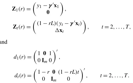
Our proposed test statistic for cases i=1, . . . ,4, denoted by˜i(1,ρ), can be constructed by following the five-step pro-¯
cedure described in this section. The test based on˜i(1,ρ)¯ is a point-optimal (invariant) test against a fixed alternativeρ= ¯ρ.
Forr∈ {1,ρ¯}, let
Step 1. Impose the null(ρ=1)and estimate the VAR
ˆ
A(L)zt(1)=dett+ ˆet, t=k+2, . . . ,T, where the deterministic terms are as according to the case under consideration and we have dropped the first observation. (We drop this observation only in this step.) From this regression, we obtain consistent estimates of the nuisance parametersandR2,
ˆ
Step 2. Estimate the coefficients φ on the deterministic terms under the null and alternative hypotheses. Each case i=1, . . . ,4 imposes a restriction of the mula for the caseiestimate is
ˆ
where[·]− is the Moore–Penrose inverse of the ar-gument.
Step 3. Construct the detrended series under the null and al-ternative hypotheses. Forr∈ {1,ρ¯}, let and construct the estimated variance–covariance ma-trices,
Step 5. Construct the test statistic as
˜
provided by Elliott and Jansson (2003) and are given in Table 1. The critical values are valid under Assumptions 1–3.
The equivalence between our testing problem and that of Elliott and Jansson (2003) enables us to use the results of that article, reinterpreted in the setting of our model, to show the up-per power bound for tests for cointegration when the cointegrat-ing vector is known and thextvariables are known to beI(1). This power bound is of practical value for two reasons. First, it gives an objective standard to compare how efficiently tests use the data. Second, it allows us to study the size of the loss in power when the cointegrating vector is not known. We under-take both of these examinations in the next section.
4. GAINS OVER ALTERNATIVE METHODS AND COMPARISON OF LOSSES FROM NOT KNOWING
THE COINTEGRATING VECTORS
The results derived earlier enable us to make a number of useful asymptotic comparisons. First, there are a number of methods available to a researcher in testing for the possibil-ity that a prespecified cointegrating vector is (under the null) not a cointegrating vector. We can directly examine the relative powers of these methods in relation to the envelope of possi-ble powers for tests. (The nonexistence of a UMP test for the hypothesis means that there is no test that has power identical to the power envelope; however, some or all of the tests may well have power close to this envelope with the implication that they are nearly efficient tests.) We examine power for various values forR2. A second comparison that can be made is exam-ination of the loss involved in estimating cointegrating vectors in testing the hypothesis that the cointegrating vector does not exist. Pesavento (2004) examined the local asymptotic power properties of a number of methods that do not require that the cointegrating vector be known. However, little is known regard-ing the extent of the loss involved in knowregard-ing or not knowregard-ing the cointegrating vector. All results are for tests with asymptotic size equal to 5%.
NOTE: Reprinted from Elliott and Jansson (2003).
4.1 Relative Powers of Tests When the Cointegrating Vector Is Known
Figures 1–4 examine the case where the cointegrating vec-tor of interest is known, and we are testing for a unit root in the cointegrating vector (null of no cointegration). As noted in Section 2, tests available for testing this null include univari-ate unit root test methods, represented here by the ADF test of Dickey and Fuller (1979) (note that theZτ test of Phillips
1987 and Phillips and Perron 1988 has the same local
asymp-(a)
(b)
(c)
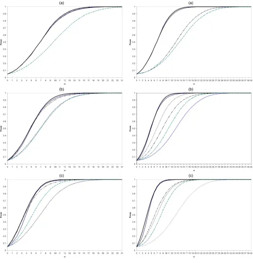
Figure 1. Asymptotic Power for (a) R2 =0 (b) R2 =.3, and
(c) R2=.5. No deterministic terms. ( EJ; CADF; PT;
ADF; ENVELOPE; HW.)
totic power) and thePTtest of Elliott et al. (1996). They also in-clude methods that exploit information in the covariates, which in addition to the test presented earlier include Hansen’s (1995) CADF test and Horvath and Watson’s (1995) Wald test. Be-cause power is influenced by the assumptions on the deter-ministics, we present results for each of the four cases for the deterministics (Figs. 1–4 are Cases 1–4). The power also de-pends on R2, the squared zero frequency correlation between the shocks driving the potentially cointegrating relation and the
Xvariables. We present three sets of results for each case.
Fig-(a)
(b)
(c)
Figure 2. Asymptotic Power, (a) R2=0 (b) R2=.3, and (c) R2=.5.
Constants, no trend. ( EJ; CADF; PT; ADF;
ENVE-LOPE; HW.)
(a)
(b)
(c)
Figure 3. Asymptotic Power, (a) R2 = 0, (b) R2 = .3, and
(c) R2=.5. Constants, no trend in the cointegrating vector. ( EJ;
CADF; PT; ADF; ENVELOPE; HW.)
ures 1(a)–1(c) are for the model with no deterministic terms withR2=0, .3, and.5 (and similarly for each of the other mod-els of the deterministic component).
When R2=0, there is no gain in using the system meth-ods over the univariate unit root methmeth-ods, because there is no exploitable information in the extra equations. In this case the Elliott and Jansson (2003) test is equivalent to thePT test, and the CADF test has equivalent power to the ADF test. This is clear from Figures 1(a), 2(a), 3(a), and 4(a), where the power curves lie on top of each other for these pairs of tests. When
(a)
(b)
(c)
Figure 4. Asymptotic Power, (a) R2 = 0, (b) R2 = .3, and
(c) R2 =.5. No restrictions in the deterministic terms. ( EJ;
CADF; PT; ADF; ENVELOPE; HW.)
there are no deterministic terms, it has previously been shown (Stock 1994; Elliott et al. 1996) that there is very little distinc-tion between the power envelope, thePTtest, and the ADF test. This is evident in Figure 1(a) which shows that all of the tests have virtually identical power curves with the power envelope. When there are deterministic terms (the remaining cases), these papers show that thePT test remains close to the power enve-lope, whereas the ADF test has lower power. This is also clear from the results in Figures 2(a), 3(a), and 4(a). As the equiva-lence between the test presented here and thePT test holds (as
does the equivalence between the CADF and ADF tests), the test presented herein has similarly better power than the CADF test.
In all cases whenR2>0,the multivariate tests have extra information to exploit. In parts (b) and (c) of Figures 1–4, we see that the power of the test presented herein is greater than that of thePT test (and the power of the CADF test is greater than that of the ADF test). As was to be expected, these dif-ferences are increasing as R2 gets larger. The differences are smaller when there is a trend in the potentially cointegrating re-lation (Case 4) than when the specification restricts such trends to be absent (Cases 1–3). There is a trade-off between using the most efficient univariate method (thePT statistic) and using the system information inefficiently [the CADF statistic and the Horvath and Watson (1995) Wald test]. Figure 2(b) shows that thePT test has power in excess of the CADF test, whereas the ranking is reversed in Figure 2(c), where the system informa-tion is stronger. In the model with a trend inβ′ztthe reversal of the ranking is already apparent whenR2=.3,implying that the relative value of the system information is larger in that case.
In all of the models, the power functions for the Elliott and Jansson (2003) tests are quite close to the power envelopes. In this sense they are nearly efficient tests. For the choices of the point alternatives suggested earlier, there is some distinction be-tween the power curve and the power envelope in the model where the cointegrating vector has a trend andR2is very large (not shown in the figures). However, this appears to be an un-likely model in practice. The power is adversely affected by less information on the deterministic terms (a common result in the unit root testing literature). We can see this clearly by holdingR2constant and looking across the figures. Comparing the constants-only model to the model with a trend in the coin-tegrating vector whenR2=.3,we have that the test achieves power at 50% forcaround 4.9 when there are constants only, whereas with trends this requires acaround 8.8,a more distant alternative. This difference essentially means that in the model with a trend in the cointegrating vector, we require about 80% more observations to achieve power at 50% against the same alternative value forρ.
Also in all models, the test presented herein has higher power than the CADF test for the null hypothesis. Again us-ing the comparisons at power equal to 50%, we have that in the model with constants only andR2=.3, we would require 80% more observations for the same power at the same value forρ. AsR2 rises, this distinction lessens. WhenR2=.5,the extra number of observations is around 60%. The distinctions are smaller when trends are possibly present. When R2=.3, we would require only 28% more observations when there is a trend in β′zt, whereas whenR2=.5, this falls to 15%. For these alternatives, the Horvath and Watson test tends to have lower power, although, as noted, this test was not designed di-rectly for this particular set of alternatives.
Overall, large power increases are available by using system tests over univariate tests except in the special case ofR2very small. Because this nuisance parameter is simply estimated, it seems that one could simply evaluate the likely power gains for a particular study using the system tests from the graphs presented.
4.2 Power Losses When the Cointegrating Vector Is Unknown
When the parameters of the cointegrating vector of interest are not specified, they are typically estimated as part of the test-ing procedure. Methods of dotest-ing this include the Engle and Granger (1987) two-step method of estimating the cointegrat-ing vector and then testcointegrat-ing the residuals for a unit root uscointegrat-ing the ADF test, and the Zivot (2000) and Boswijk (1994) tests in the error-correction models. One could also simply use a rank test, testing the null hypothesis of m+1 unit roots ver-susmunit roots. These tests include the Johansen (1988, 1995) and Johansen and Juselius (1990) methods and the Harbo et al. (1998) rank test in partial systems. The Zivot (2000) test is equivalent to thet-test of Banerjee, Dolado, Hendry, and Smith (1986) and Banerjee, Dolado, Galbraith, and Hendry (1993) in a conditional ECM with unknown cointegration vector (denoted by ECR thereafter). In addition, for the case examined in this article in which the right side variables are not mutually coin-tegrated and there is at most one cointegration vector, the rank test of Harbo, Johansen, Nielsen, and Rahbek (1998) is equiva-lent to the Wald test of Boswijk (1994). The rank tests are not derived under the assumption thatxtisI(1), implying that they spread power (in an arbitrary and random way) among the al-ternatives that we examine here as well as alal-ternatives in the direction of one (or more) of thextvariables being stationary. Although the rank tests do not make optimal use of the infor-mation aboutxt,these tests will, of course, still be consistent against the alternatives considered in this article. We demon-strate numerically that the failure to impose the information onxtcomes at a relatively high cost.
Pesavento (2004) gave a detailed account of the aforemen-tioned methods and computed power functions for tests of the null hypothesis that there is no cointegrating vector. The pow-ers of the tests are found to depend asymptotically on the specification of the deterministic terms and R2,just as in the known cointegrating vector case. Pesavento (2004) found that the ECMs outperform the other methods for all models, and the ranking between the Engle and Granger (1987) method and the Johansen (1988, 1995) methods depends on the value for R2, with the first method (a univariate method) being useful when there is little extra information in the remaining equations of the system (i.e., whenR2is small) and the Johansen full-system method being better when the amount of extra exploitable infor-mation is substantial.
The absolute loss from not knowing the cointegrating vec-tor can be assessed by examining the difference between the power envelope when the cointegrating vector is known versus the power functions for these tests. The quantification of this gap is useful for researchers in examining results where one estimates the cointegrating vector even though theory specifies the coefficients of the vector (a failure to reject may be due to a large decrease in power), and also can provide guidance for test-ing in practice when one has a vector and does not know if they should specify it for the test. In this case, if the power losses are small, then it would be prudent to not specify the coefficients of the cointegrating vector, but instead estimate it.
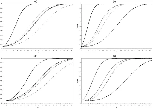
Figures 5–7 show the results for these power functions for values forR2=0, .3,and.5. Each figure has two panels, (a) for
(a)
(b)
Figure 5. Asymptotic Power Known and Unknown Cointegration
Vector, R2=0, (a) Constants, No Trend, and (b) No Restrictions
in the Deterministic Terms. ( Envelope-Case2; EG-Case2;
Zivot/ECR-Case2; Johansen-Case2; Wald/Harbo-Case2.)
the model with constants only and (b) for the model with a trend in the cointegrating vector. The first point to note is that in all cases, the gap between the power envelope when the
coeffi-(a)
(b)
Figure 7. Asymptotic Power Known and Unknown Cointegration
Vec-tor, R2=.5, (a) Constants, No Trend, and (b) No Restrictions in
the Deterministic Terms. ( Envelope-Case2; EG-Case2;
Zivot/ECR-Case2; Johansen-Case2; Wald/Harbo-Case2.)
cients of the cointegrating vector are known and the best test is very large. This means that there is a large loss in power from estimating the cointegrating vector. Comparing panels
(a) (b)
Figure 6. Asymptotic Power Known and Unknown Cointegration Vector, R2=.3, (a) Constants, No Trend, and (b) No Restrictions in the
Deter-ministic Terms. ( Envelope-Case2; EG-Case2; Zivot/ECR-Case2; Johansen-Case2; Wald/Harbo-Case2.)
(a) and (b) for each of these figures, we see that additional deter-ministic terms (trend vs. constant) results in a smaller gap. This is most apparent whenR2=0 and lessens asR2gets larger. In Case 2, when R2=.3 [Fig. 6(a)] at c= −5, we have power of 53% for the power envelope and just 13% for the best test examined that does not have the coefficients of the cointegrat-ing vector known (the ECR test). In Case 2 withR2=.3,we have that atc= −5, the envelope is 53%, but the power of the ECR test is 13%, as noted earlier. For the model with trends, the envelope is 24% and the power of the ECR test is 8%. The dif-ference falls from 40% to 16%. In general, for the model with trends, the power curves tend to be closer together than in the constants-only, model compressing all of the differences.
As R2 rises, the gap between the power envelope and the power of the best test falls. This is true for both cases. In the constants-only model whenR2=0, we have at c= −10, we have 79% power for the envelope and 27% power for the ECR test. When R2 increases to .5, we have power for the enve-lope of 98% and 54% for the ECR test. The difference falls from 52% to 44%.
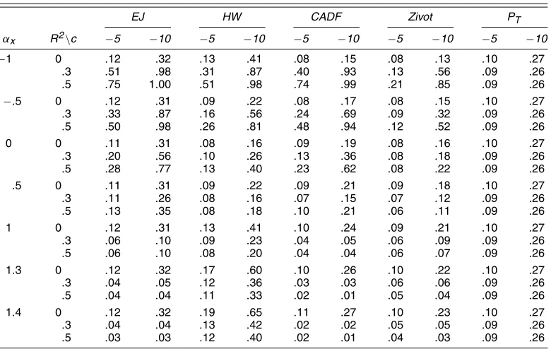
4.3 Power of the Test Whenαx Is Different From 0 in (5)
Although the assumption thatxt isI(1)under both the null and local alternative is a reasonable assumption in the context of cointegration, we can also examine the sensitivity of the pro-posed tests to different values ofαxin (5). Recall that for these modelsxt isI(1)under the null but under the alternative has a small additional local toI(2)component. We simulate (5) with scalarxtandβ=(1,−1)′, parameter that determines asymptotic power (whenαx=0).
The system can be written as
(yt−xt)=(ρ−1)(1−Rαx)(yt−1−xt−1) then the error-correction term,yt−1,is not mean-reverting, and
tests based on (9) will be inconsistent (see also Zivot 2000,
p. 429). For this reason, we consider only values for αx such thatRαx<1.
The number of lags (one) is assumed known [for the Hansen (1995) and Zivot (2000) tests, one lead ofxtis also included]. The regressions are estimated for the models with no determin-istic terms, with constants only and with no restrictions. We do not report results for case 3, because they are similar to the included results. The sample size is T =1,500, and we used 10,000 replications.
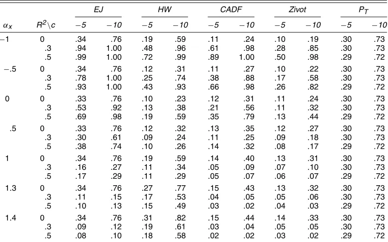
Tables 2–4 report the rejection rates for various values ofαx. The rejection rates forc=0 do not vary withαxand are not re-ported, because they equal.05.Whenαx=0,the power of the Elliott and Jansson (2003) test is higher than the power of any other tests, including the Horvath and Watson (1995) test. In the simulated data-generated process,Ais not lower triangular, soαx=0 does not coincide with weak exogeneity. The Elliott and Jansson (2003) test exploits the information contained in the covariates in an optimal way and thus rejects the null hy-pothesis with higher probability than the Horvath and Watson (1995) test.
Whenαxis positive, the root ofytin (9) is larger (in our sim-ulationsωxyis positive, soRαx>0), so all of the tests based on (9) will have smaller power, as will the test proposed herein. For positive but small values ofαx,the Elliott and Jansson (2003) test still performs relatively well compared with other tests. Only when there are no deterministic terms andR2is 0 does the proposed test reject a false null with probability smaller than Hansen’s (1995) CADF test. Asαx increases, the Horvath and Watson (1995) trace test outperforms the other tests in most cases. When the deterministic terms include a constant but not a trend, the Elliott and Jansson (2003) test has power similar to the Horvath and Watson (1995) test in a neighborhood of the null.
ThePT test of Elliott et al. (1996) does not use the informa-tion in the covariates, and the power forαx=0 is lower than that of the Elliott and Jansson (2003) test whenR2is different than 0. Given that thePT test is based on the single equation, it is not sensitive to αx and it rejects with higher probability than the Elliott and Jansson (2003) test for large positive values ofαx whenR2 is positive. Finally, the test proposed by Zivot (2000) rejects the null with lower probability than the Elliott and Jansson (2003) test for any value ofαx.This is not surpris-ing given that Zivot’s test does not fully utilize the information that the cointegrating vector is known.
Whenαx is negative, the coefficient for the error-correction term in the conditional equation is forther away from 0, and all of tests reject the null of no cointegration more often with the Elliott and Jansson (2003) test having the highest power as soon asR2departs from 0.
4.4 Small-Sample Comparisons
The results of the previous sections show that the Elliott and Jansson (2003) family of tests has optimality properties when applied in the context of model (1)–(3) and has asymptotic power that depends on the nuisance parameter R2. Although the particular estimator used to estimate the nuisance parame-ters does not affect the asymptotic distributions under the local alternatives, the finite-sample properties of tests for no cointe-gration can be sensitive to the choice of the estimation method.
Table 2. Rejection Rates Whenαx=0 in (5), No Deterministic Terms
EJ HW CADF Zivot PT
αx R2\c −5 −10 −5 −10 −5 −10 −5 −10 −5 −10
−1 0 .33 .76 .43 .89 .28 .63 .14 .32 .30 .73
.3 .93 1.00 .82 1.00 .93 1.00 .50 .98 .29 .72
.5 .99 1.00 .94 1.00 .99 1.00 .76 1.00 .29 .72
−.5 0 .33 .76 .25 .64 .30 .69 .16 .38 .30 .73
.3 .77 .99 .56 .95 .78 .99 .32 .86 .29 .72
.5 .93 1.00 .77 .99 .92 1.00 .49 .96 .29 .72 0 0 .33 .76 .18 .49 .32 .75 .18 .45 .30 .73
.3 .51 .92 .29 .72 .50 .90 .21 .58 .29 .72
.5 .68 .98 .43 .88 .67 .96 .25 .72 .29 .72
.5 0 .33 .76 .25 .64 .35 .81 .19 .48 .30 .73
.3 .29 .61 .18 .49 .26 .57 .14 .31 .29 .72
.5 .36 .73 .20 .54 .31 .61 .13 .30 .29 .72 1 0 .33 .76 .44 .89 .39 .86 .19 .50 .30 .73
.3 .15 .26 .26 .66 .13 .25 .08 .14 .29 .72
.5 .16 .27 .22 .59 .11 .17 .06 .09 .29 .72 1.3 0 .33 .76 .59 .97 .41 .88 .19 .51 .30 .73
.3 .10 .14 .39 .85 .09 .14 .06 .08 .29 .72
.5 .10 .12 .36 .82 .05 .06 .04 .04 .29 .72 1.4 0 .33 .76 .64 .98 .42 .89 .19 .52 .30 .73
.3 .09 .11 .44 .89 .08 .12 .05 .06 .29 .72
.5 .08 .09 .42 .88 .04 .04 .03 .03 .29 .72
To study the small-sample behavior of the proposed test, we simulate (5) with scalarxt, αx=0,andβ=(1,−1)′,
(yt−xt)=(ρ−1)(yt−1−xt−1)+vy,t and
xt=vx,t.
The error process vt = (vy,t,vx,t)′ is generated by the VARMA(1, 1) model
(I2−AL)vt=(I2+L)εt,
where
A=
a1a2 a2a1
, =
θ1θ2
θ2θ1
,
andεt∼iidN(0,), whereis chosen in such a way that the long-run variance–covariance matrix ofvtsatisfies
=(I2−A)−1(I2+)(I2+)′(I2−A)−1′
=
1 R R 1
, R∈ [0,1).
Table 3. Rejection Rates Whenαx=0 in (5), Constants, No Trend
EJ HW CADF Zivot PT
αx R2\c −5 −10 −5 −10 −5 −10 −5 −10 −5 −10
−1 0 .34 .76 .19 .59 .11 .24 .10 .19 .30 .73
.3 .94 1.00 .48 .96 .61 .98 .28 .85 .30 .73
.5 .99 1.00 .72 .99 .89 1.00 .50 .98 .29 .72
−.5 0 .34 .76 .12 .31 .11 .27 .10 .22 .30 .73
.3 .78 1.00 .25 .74 .38 .88 .17 .58 .30 .73
.5 .93 1.00 .43 .93 .66 .98 .26 .82 .29 .72 0 0 .33 .76 .10 .23 .12 .31 .11 .24 .30 .73
.3 .53 .92 .13 .38 .21 .56 .11 .32 .30 .73
.5 .69 .98 .19 .59 .35 .79 .13 .44 .29 .72
.5 0 .33 .76 .12 .32 .13 .35 .12 .27 .30 .73
.3 .30 .61 .09 .24 .11 .25 .09 .18 .30 .73
.5 .38 .74 .10 .26 .14 .32 .08 .17 .29 .72 1 0 .34 .76 .19 .59 .14 .40 .13 .31 .30 .73
.3 .16 .27 .11 .34 .05 .09 .07 .10 .30 .73
.5 .17 .29 .11 .29 .05 .07 .06 .07 .29 .72 1.3 0 .34 .76 .27 .77 .15 .43 .13 .32 .30 .73
.3 .11 .15 .17 .53 .04 .05 .05 .06 .30 .73
.5 .10 .13 .15 .49 .03 .02 .04 .03 .29 .72 1.4 0 .34 .76 .31 .82 .15 .44 .14 .33 .30 .73
.3 .09 .12 .19 .61 .03 .04 .05 .05 .30 .73
.5 .08 .10 .18 .58 .02 .02 .03 .02 .29 .72
Table 4. Rejection Rates Whenαx=0 in (5), No Restrictions
EJ HW CADF Zivot PT
αx R2\c −5 −10 −5 −10 −5 −10 −5 −10 −5 −10
−1 0 .12 .32 .13 .41 .08 .15 .08 .13 .10 .27
.3 .51 .98 .31 .87 .40 .93 .13 .56 .09 .26
.5 .75 1.00 .51 .98 .74 .99 .21 .85 .09 .26
−.5 0 .12 .31 .09 .22 .08 .17 .08 .15 .10 .27
.3 .33 .87 .16 .56 .24 .69 .09 .32 .09 .26
.5 .50 .98 .26 .81 .48 .94 .12 .52 .09 .26 0 0 .11 .31 .08 .16 .09 .19 .08 .16 .10 .27
.3 .20 .56 .10 .26 .13 .36 .08 .18 .09 .26
.5 .28 .77 .13 .40 .23 .62 .08 .22 .09 .26
.5 0 .11 .31 .09 .22 .09 .21 .09 .18 .10 .27
.3 .11 .26 .08 .16 .07 .15 .07 .12 .09 .26
.5 .13 .35 .08 .18 .10 .21 .06 .11 .09 .26 1 0 .12 .31 .13 .41 .10 .24 .09 .21 .10 .27
.3 .06 .10 .09 .23 .04 .05 .06 .09 .09 .26
.5 .06 .10 .08 .20 .04 .04 .06 .07 .09 .26 1.3 0 .12 .32 .17 .60 .10 .26 .10 .22 .10 .27
.3 .04 .05 .12 .36 .03 .03 .06 .06 .09 .26
.5 .04 .04 .11 .33 .02 .01 .05 .04 .09 .26 1.4 0 .12 .32 .19 .65 .11 .27 .10 .23 .10 .27
.3 .04 .04 .13 .42 .02 .02 .05 .05 .09 .26
.5 .03 .03 .12 .40 .02 .01 .04 .03 .09 .26
We estimated the number of lags and leads by the Bayesian information criterion on a VAR on the first differences (under the null) with a maximum of eight lags. For Case 2, we esti-mated the regressions with a mean. For the model with a trend in the cointegrating vector, we estimated the regressions with a mean and a trend; results for other cases were similar. The sample size isT=100, and we used 10,000 replications.
Tables 5 and 6 compare the small sample size of the Elliott and Jansson (2003) test and Hansen (1995) CADF test for var-ious values ofandA. To compute the critical values in each case, we estimated the value ofR2as suggested by Elliott and Jansson (2003) and Hansen (1995). Overall, the Elliott and Jansson (2003) test is worse in terms of size performance than the CADF test. This is the same type of difference found be-tween thePT and DF tests in the univariate case, and so is not surprising given that these methods are extensions of the two univariate tests. The difference between the two tests is more evident for large values ofR2and for the case with no trend. Whenis nonzero, both tests present size distortions that are severe in the presence of a large negative moving average root (as is the case for unit root tests), emphasizing the need for proper modeling of the serial correlation present in the data.
5. COINTEGRATION BETWEEN FORECASTS AND OUTCOMES
There are a number of situations where if there is a cointe-grating vector, then we have theory that suggests the form of the cointegrating vector. In the purchasing power parity literature, the typical assumption is that logs of the nominal exchange rate and home and foreign prices all have unit roots and the real exchange rate does not. The real exchange rate is constructed from theI(1)variables with the cointegrating vector(1,1,−1)′. In examining interest rates, we find that term structure theories often imply a cointegrating structure of (1,−1)′ between in-terest rates of different maturities; however, one might find it difficult to believe that the log interest rate is unbounded, and hence is unlikely to have a unit root.
Another example involves the forecasts and outcomes of the variable of interest. Because many variables that macro-economists would like to forecast have trending behavior, often taken to be unit root behavior, some researchers have examined whether or not the forecasts made in practice are indeed coin-tegrated with the variable being forecast. The expected cointe-grating vector is(1,−1)′,implying that the forecast error is sta-tionary. This has been undertaken for exchange rates (Liu and
Table 5. Small Sample Size, Constants, No Trend
A Θ EJ CADF
a1 a2 θ1 θ2 R2=0 R2=.3 R2=.5 R2=0 R2=.3 R2=.5
0 0 0 0 .059 .070 .074 .051 .055 .058
.2 0 0 0 .060 .077 .089 .047 .058 .062
.8 0 0 0 .066 .083 .103 .075 .085 .086
.2 .5 0 0 .089 .078 .076 .104 .069 .059 0 0 −.2 0 .104 .112 .113 .077 .068 .061 0 0 .8 0 .106 .152 .207 .057 .063 .067 0 0 −.5 0 .167 .169 .189 .102 .082 .068 0 0 −.8 0 .352 .341 .372 .256 .197 .144
.2 0 −.5 0 .160 .166 .181 .104 .085 .070
Table 6. Small Sample Size, No Restrictions
A Θ EJ CADF
a1 a2 θ1 θ2 R2=0 R2=.3 R2=.5 R2=0 R2=.3 R2=.5
0 0 0 0 .048 .054 .057 .055 .051 .052
.2 0 0 0 .037 .052 .062 .039 .051 .059
.8 0 0 0 .043 .088 .143 .083 .091 .100
.2 .5 0 0 .061 .057 .060 .142 .082 .063 0 0 −.2 0 .098 .104 .123 .091 .073 .064 0 0 .8 0 .057 .122 .207 .059 .067 .075 0 0 −.5 0 .173 .187 .219 .131 .097 .082 0 0 −.8 0 .371 .324 .350 .299 .232 .176
.2 0 −.5 0 .161 .148 .153 .134 .100 .080
Maddala 1992) and macroeconomic data (Aggarwal, Mohanty, and Song 1995). In the context of macroeconomic forecasts, Cheung and Chinn (1999) also relaxed the cointegrating vector assumption.
The requirement that forecasts be cointegrated with out-comes is a very weak requirement. Note that the forecaster’s information set includes the current value of the outcome vari-able. Because the current value of the outcome variable is trivially cointegrated with the future outcome variable to be forecast (they differ by the change, which is stationary), the forecaster has a simple observable forecast that satisfies the requirement that the forecast and outcome variable be cointe-grated. We can also imagine what happens under the null hy-pothesis of no cointegration. Under the null, forecast errors are
I(1)and hence become arbitrarily far from 0 with probability 1. It is hard to imagine that a forecaster would stick with such a method when the forecast gets further away from the current value of the outcome than typical changes in the outcome vari-able would suggest are plausible.
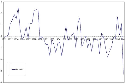
This being said, of course it is useful if tests reject the hy-pothesis of no cointegration and is quite indicative of power problems if they do not. Here we use forecasts of the price level from the Livingston dataset over the period 1971–2000. The survey recipients forecast the consumer price index 6 months ahead. Figure 8 shows the forecast errors. Because the vari-ables are indexes, a value of 1 is a 1% difference relative to the base of 1982–1984. Forecast errors at different times have been quite large, especially around the times of the oil shocks in the 1970s. They have been smaller and more often negative
Figure 8. Forecast Errors for 6-Months-Ahead Forecasts.
over the last two decades—this was a period of falling inflation rates that appears to have induced the error on average of over-estimating prices. There is no indication from the data that the errors are getting larger in variance over time, although there are long swings in the forecast error that may lead lower-power tests into failing to reject the hypothesis that the forecast error does not have a unit root.
Indeed, the Dickey and Fuller (1979) test is unable to reject a unit root in the forecast error, even at the 10% level. This is shown in Table 7, which provides the results of the test in column 1. We have allowed for a nonzero mean under the al-ternative (i.e., the constant included case of the test). Com-monly used multivariate tests do a little better. The Horvath and Watson (1995) test fails to reject at the 10% level, whereas the CADF test rejects at the 5% level but not at the 1% level. Thus, even though the null hypothesis is an extremely weak re-quirement of the data, the forecasts fail the test in most cases. However, the problem could be one of power rather than of ex-tremely poor forecasting. This is further backed up by the tests of Elliott et al. (1996), which reject at the 5% level but not at the 1% level. Thepvalue for thePT test is .02.
The first two columns of Table 8 presents results for the Elliott and Jansson (2003) test under the assumption that the change in the forecasts is on the right side of the cointegrating regression. OurX variable is chosen to be price expectations. Results are similar when prices are chosen as theXvariable, as reported in Table 8. We examine Case 3, that is, the statistic is invariant to a mean in the change in forecasts (so that this vari-able has a drift, prices rise over time, suggesting a positive drift) and a mean in the quasi-difference of the cointegrating vector under the alternative. For there to be gains over univariate tests, theR2 value should be different from 0. Here we estimateR2
to be .19, suggesting that there are gains from using this mul-tivariate approach. Comparing the statistic developed here with its critical value, we are able to reject not only at the 5% level, but also at the 1% level. Comparing this results with those for the previous tests, we see results that we may have expected from the asymptotic theory. Standard unit root tests have low
Table 7. Cointegration Tests
ADF HW CADF PT DF–GLS
Forecast errors −2.72 7.43 −2.48∗ 2.38∗ −2.72∗ (2) (2) (2) (2)
NOTE: The number of lags was chosen by MAIC and is reported in parentheses.
∗Significance at 5%.
Table 8. Cointegration Tests, Stationary Covariate
EJ, Case 3,∆petcov Rˆ2 EJ, Case 3,∆ptcov Rˆ2
Forecast errors .60∗∗ .60∗∗
(2) .19 (1) .10
pvalue .003 .001
NOTE: The first two columns give results for tests whereXt=pet; the remaining two columns give results forXt=pt.
∗∗Significance at 1%.
power (and we do not reject with the Dicken–Fuller test). We can improve power by using additional information, such as us-ing CADF, or by usus-ing the data more efficiently throughPT. In these cases we do reject at the 5% level. Finally, using the addi-tional information and using all information efficiently, where we expect to have the best power, we reject not only at the 5% level, but also at the 1% level. We are able to reject that the cointegrating vector has a unit root and conclude that the fore-cast errors are indeed mean-reverting, a result that is not avail-able with current multivariate tests and is less assured from the higher-power univariate tests.
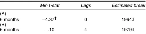
As a robustness check, we also tested the data for a unit root allowing for a break at unknown time. The forecast errors in Figure 8 appear to have a shift in the level around 1980–1983 that could lower the probability of rejection of conventional tests. To test the data for a unit root with break, we use the test of Perron and Vogelsang (1992). LetDUt=1 ift>Tband 0 otherwise, whereTbis the break date. Following Perron and Vogelsang (1992), we first remove the deterministic part of the series for a given breakTbby estimating the regression
yt=µ+δDUt+yt.
Panel A in Table 9 corresponds to the case in which the break is estimated as the date that minimizes thet-statisticstσˆ in the unit root test. The number of lags is chosen for a given break such that the coefficient on the last included lag of the first dif-ferences of the data is significant at 10% level (for details, see Perron and Vogelsang 1992). Panel B corresponds to the case in which the break is chosen to minimize thet-statistics testing δ=0 in the first regression.
Table 9. Unit Root Test With Breaks
Min t-stat Lags Estimated break
(A)
6 months −4.37† 0 1994:II (B)
6 months −.10 4 1979:II
NOTE: Panel A corresponds to the case in which the break is estimated as the date that minimizes thet-statistics in the unit root test, Panel B corresponds to the case in which the break is chosen to minimize thet-statistics testing in the break regression (see Perron and Vogelsang 1992). The small sample 5% and 10% critical values that take into account the lag selection procedure are−4.67 and−4.33 for Panel A and−3.68 and−3.35 for Panel B.
†Rejection at 10%.
As the table shows, standard methods reject for some cases but not everywhere. When the break is chosen to minimize the
t-statistic in the unit root test, the unit root with break test re-jects at 10% level. When the break is chosen as the date that minimizes thet-statistic in the regression for the deterministic, we cannot reject the unit root hypothesis. Overall, it appears that if there is a break, it is small. This is all the more reason to use tests that use the data as efficiently as possible.
6. CONCLUSION
In this article we have examined the idea of testing for a unit root in a cointegrating vector when the cointegrating vector is known and the variables are known to be I(1). Early studies simply performed unit root tests on the cointegrating vector; however, this approach omits information that can be very use-ful in improving the power of the test for a unit root. The re-strictions placed on the multivariate model for this “known a priori” information renders the testing problem equivalent to that of Elliott and Jansson (2003), and so we use those tests here. Whereas there exists no UMP test for the problem, the point-optimal tests derived by Elliott and Jansen (2003) and ap-propriate here are among the asymptotically admissible class (because they are asymptotically equivalent to the optimal test under normality at a point in the alternative) and were shown to perform well in general.
The method is quite simple, requiring the running of a VAR to estimate nuisance parameters, detrending the data (under both the null and the alternative), and then running two VARs, one on the data detrended under the null and another based on the data detrended under the alternative. The statistic is then constructed from the variance–covariance matrices of the resid-uals of these VARs.
We then applied the method to examine the cointegration of forecasts of the price level with the actual price levels. The idea that forecasts and their outcomes are cointegrated with cointe-grating vector (1,−1)′ (so forecast errors are stationary) is a very weak property. It is difficult to see that such a property could be violated by any serious forecaster. The data we exam-ine here comprise 6-month-ahead forecasts from the Livingston data for prices for 1971–2000. However, most simple univariate tests and some of the more sophisticated multivariate tests cur-rently available to test the proposition do not reject the null that the forecast errors have a unit root. The tests derived here are able to reject this hypothesis with a great degree of certainty.
ACKNOWLEDGMENT
The authors thank two anonymous referees and an associate editor for helpful comments.
APPENDIX: NOTES ON THE DATA
The current CPI is the non–seasonally adjusted CPI for all Urban Consumers from the Bureau of Labor and Statistics (code CUUR0000SA0) corresponding to the month being fore-casted. All the current values for the CPI are in 1982–1984 base year.
The forecasts CPI data are the 6-month price forecasts from the Livingston Tables at the Philadelphia Fed from June 1971 to December 2001. The survey is conducted twice a year (early June and early December) to obtain the 6-month-ahead fore-casts from a number of respondents. The number of respondents varies for each survey, so each forecast in our sample is com-puted as the average of the forecasts from all the respondents from each survey. The data in the Livingston Tables are avail-able in the 1967 base up to December 1987 and the 1982–1984 base thereafter. Given that there are not overlapping forecasts at both base years, we transformed all of the forecasts to the 1982–1984 base as follows. We first computed the average of the actual values for the 1982–1984 base CPI for the year 1967, then used this value to multiply all the forecasts before 1987 to transform the forecasts to the 1982–1984 base.
At the time of the survey, the respondents were also given current figures on which to base their forecasts. The surveys are sent out early in the month, so the available information to the respondents for the June and December survey are April and October. For this reason, although traditionally the forecasts are called 6-month-ahead forecasts, they are truly 7-month-ahead forecasts. Carlson (1977) presented a detailed description of the issues related to the price forecasts from the Livingston Survey.
[Received August 2002. Revised May 2004.]
REFERENCES
Aggarwal, R., Mohanty, S., and Song, F. (1995), “Are Survey Forecasts of Macroeconomic Variables Rational?”Journal of Business, 68, 99–119. Banerjee, A., Dolado, J., Galbraith, J. W., and Hendry, D. F. (1993),
Co-Integration, Error Correction, and the Econometric Analysis of Non-Stationary Data, Oxford, U.K.: Oxford University Press.
Banerjee, A., Dolado, J., Hendry, D. F., and Smith, G. W. (1986), “Explor-ing Equilibrium Relationship in Econometrics Through Static Models: Some Monte Carlo Evidence,”Oxford Bulletin of Economics and Statistics, 48, 253–277.
Bernard, A., and Durlauf, S. (1995), “Convergence in International Output,”
Journal of Applied Econometrics, 10, 97–108.
Boswijk, H. P. (1994), “Testing for an Unstable Root in Conditional and Struc-tural Error Correction Models,”Journal of Econometrics, 63, 37–60. Carlson, J. A. (1977), “A Study of Price Forecasts,”Annals of Economic and
Social Measurement, 6, 27–56.
Cheung, Y.-W., and Chinn, M. D. (1999), “Are Macroeconomic Forecasts Infor-mative? Cointegration Evidence From the ASA–NBER Surveys,” Discussion Paper 6926, National Bureau of Economic Research.
Cheung, Y.-W., and Lai, K. (2000), “On Cross-Country Differences in the Per-sistence of Real Exchange Rates,”Journal of International Economics, 50, 375–397.
Cox, D. R., and Hinkley, D. V. (1974),Theoretical Statistics, New York: Chap-man & Hall.
Dickey, D. A., and Fuller, W. A. (1979), “Distribution of Estimators for Autore-gressive Time Series With a Unit Root,”Journal of the American Statistical Association, 74, 427–431.
Elliott, G., and Jansson, M. (2003), “Testing for Unit Roots With Stationary Covariates,”Journal of Econometrics, 115, 75–89.
Elliott, G., Rothenberg, T. J., and Stock, J. H. (1996), “Efficient Tests for an Autoregressive Unit Root,”Econometrica, 64, 813–836.
Engle, R. F., and Granger, C. W. J. (1987), “Cointegration and Error Correction: Representation, Estimation and Testing,”Econometrica, 55, 251–276. Greasley, D., and Oxley, L. (1997), “Time–Series Based Tests of the
Conver-gence Hypothesis: Some Positive Results,”Economics Letters, 56, 143–147. Hansen, B. E. (1995), “Rethinking the Univariate Approach to Unit Root Testing: Using Covariates to Increase Power,” Econometric Theory, 11, 1148–1171.
Harbo, I., Johansen, S., Nielsen, B., and Rahbek, A. (1998), “Asymptotic In-ference on Cointegrating Rank in Partial Systems,”Journal of Business & Economic Statistics, 16, 388–399.
Horvath, M. T. K., and Watson, M. W. (1995), “Testing for Cointegration When Some of the Cointegrating Vectors Are Prespecified,”Econometric Theory, 11, 984–1014.
Johansen, S. (1988), “Statistical Analysis of Cointegration Vectors,”Journal of Economic Dynamics and Control, 12, 231–254.
(1995),Likelihood-Based Inference in Cointegrated Autoregressive Models, Oxford, U.K.: Oxford University Press.
Johansen, S., and Juselius, K. (1990), “Maximum Likelihood Estimation and Inference on Cointegration With Application to the Demand for Money,” Ox-ford Bulletin of Economics and Statistics, 52, 169–210.
King, M. L. (1988), “Towards a Theory of Point Optimal Testing,”Econometric Reviews, 6, 169–218.
Kremers, J. J. M., Ericsson, N. R., and Dolado, J. (1992), “The Power of Coin-tegration Tests,”Oxford Bulletin of Economics and Statistics, 54, 325–348. Liu, T., and Maddala, G. S. (1992), “Rationality of Survey Data and Tests for
Market Efficiency in the Foreign Exchange Markets,”Journal of Interna-tional Money and Finance, 11, 366–381.
Perron, P., and Vogelsang, T. J. (1992), “Non-Stationarity and Level Shifts With an Application to Purchasing Power Parity,”Journal of Business & Economic Statistics, 10, 301–320.
Pesavento, E. (2004), “An Analytical Evaluation of the Power of Tests for the Absence of Cointegration,”Journal of Econometrics, 122, 349–384. Phillips, P. C. B. (1987), “Time Series Regression With a Unit Root,”
Econo-metrica, 55, 277–301.
Phillips, P. C. B., and Perron, P. (1988), “Testing for a Unit Root in Time Series Regression,”Biometrika, 75, 335–346.
Phillips, P. C. B., and Solo, V. (1992), “Asymptotic for Linear Processes,”
The Annals of Statistics, 20, 971–1001.
Rothenberg, T. J., and Stock, J. H. (1997), “Inference in a Nearly Integrated Au-toregressive Model With Nonnormal Innovations,”Journal of Econometrics, 80, 269–286.
Stock, J. H. (1994), “Unit Roots, Structural Breaks and Trends,” inHandbook of Econometrics, Vol. IV, eds. R. F. Engle and D. L. McFadden, New York: North-Holland, pp. 2739–2841.
Zivot, E. (2000), “The Power of Single Equation Tests for Cointegration When the Cointegrating Vector Is Prespecified,”Econometric Theory, 16, 407–439.