molecular modelling for beginners

(1)

Molecular Modelling

for Beginners

(2)

(3)

(4)

(5)

Molecular Modelling

for Beginners

(6)

National 01243 779777 International (þ44) 1243 779777

E-mail (for orders and customer service enquiries): cs-books@wiley.co.uk Visit our Home Page on www.wileyeurope.com

or www.wiley.com

All Rights Reserved. No part of this publication may be reproduced, stored in a retrieval system or transmitted in any form or by any means, electronic, mechanical, photocopying, recording, scanning or otherwise, except under the terms of the Copyright, Designs and Patents Act 1988 or under the terms of a licence issued by the Copyright Licensing Agency Ltd, 90 Tottenham Court Road, London W1P 4LP, UK, without the permission in writing of the Publisher. Requests to the Publisher should be addressed to the Permissions Department, John Wiley & Sons Ltd, The Atrium, Southern Gate, Chichester, West Sussex PO19 8SQ, England, or emailed to permreq@wiley.co.uk, or faxed to (þ44) 1243 770620.

This publication is designed to provide accurate and authoritative information in regard to the subject matter covered. It is sold on the understanding that the Publisher is not engaged in rendering professional services. If professional advice or other expert assistance is required, the services of a competent professional should be sought.

Other Wiley Editorial Offices

John Wiley & Sons Inc., 111 River Street, Hoboken, NJ 07030, USA Jossey-Bass, 989 Market Street, San Francisco, CA 94103-1741, USA Wiley-VCH Verlag GmbH, Boschstr. 12, D-69469 Weinheim, Germany

John Wiley & Sons Australia Ltd, 33 Park Road, Milton, Queensland 4064, Australia

John Wiley & Sons (Asia) Pte Ltd, 2 Clementi Loop #02-01, Jin Xing Distripark, Singapore 129809 John Wiley & Sons Canada Ltd, 22 Worcester Road, Etobicoke, Ontario, Canada M9W 1L1

Wiley also publishes its books in a variety of electronic formats. Some content that appears in print may not be available in electronic books.

Library of Congress Cataloging-in-Publication Data (to follow)

British Library Cataloguing in Publication Data

A catalogue record for this book is available from the British Library ISBN 0 470 84309 8 (Hardback)

0 470 84310 1 (Paperback)

Typeset in 10.5=13pt Times by Thomson Press (India) Ltd., Chennai

Printed and bound in Great Britain by TJ International Ltd., Padstow, Cornwall

(7)

Preface

There is nothing radically new about the techniques we use in modern molecular modelling. Classical mechanics hasn’t changed since the time of Newton, Hamilton and Lagrange, the great ideas of statistical mechanics and thermodynamics were discovered by Ludwig Boltzmann and J. Willard Gibbs amongst others and the basic concepts of quantum mechanics appeared in the 1920s, by which time J. C. Maxwell’s famous electromagnetic equations had long since been published.

The chemically inspired idea that molecules can proﬁtably be treated as a collec-tion of balls joined together with springs can be traced back to the work of D. H. Andrews in 1930. The ﬁrst serious molecular Monte Carlo simulation appeared in 1953, closely followed by B. J. Alder and T. E. Wainwright’s classic molecular dynamics study of hard disks in 1957.

The Hartrees’ 1927 work on atomic structure is the concrete reality of our everyday concept of atomic orbitals, whilst C. C. J. Roothaan’s 1951 formulation of the HF–LCAO model arguably gave us the basis for much of modern molecular quantum theory.

If we move on a little, most of my colleagues would agree that the two recent major advances in molecular quantum theory have been density functional theory, and the elegant treatment of solvents using ONIOM. Ancient civilizations believed in the cyclical nature of time and they might have had a point for, as usual, nothing is new. Workers in solid-state physics and biology actually proposed these models many years ago. It took the chemists a while to catch up.

Scientists and engineers ﬁrst got their hands on computers in the late 1960s. We have passed the point on the computer history curve where every 10 years gave us an order of magnitude increase in computer power, but it is no coincidence that the growth in our understanding and application of molecular modelling has run in parallel with growth in computer power. Perhaps the two greatest driving forces in recent years have been the PC and the graphical user interface. I am humbled by the fact that my lowly 1.2 GHz AMD Athlon ofﬁce PC is far more powerful than the world-beating mainframes that I used as a graduate student all those years ago, and that I can build a molecule on screen and run a B3LYP/6-311þþG(3d, 2p) calcula-tion before my eyes (of which more in Chapter 20).

(16)

produce the screenshots; obviously they look better in colour than the greyscale of this text.

There are a number of classic (and hard) texts in the ﬁeld; if I’m stuck with a basic molecular quantum mechanics problem, I usually reach for Eyring, Walter and Kimball’sQuantum Chemistry, but the going is rarely easy. I make frequent mention of this volume throughout the book.

Equally, there are a number of beautifully produced elementary texts and software reference manuals that can apparently transform you into an expert overnight. It’s a two-edged sword, and we are victims of our own success. One often meets self-appointed experts in the ﬁeld who have picked up much of the jargon with little of the deep understanding. It’s no use (in my humble opinion) trying to hold a con-versation about gradients, hessians and density functional theory with a colleague who has just run a molecule through one package or another but hasn’t the slightest clue what the phrases or the output mean.

It therefore seemed to me (and to the Reviewers who read my New Book Proposal) that the time was right for a middle course. I assume that you are a ‘Beginner’ in the sense ofChambers Dictionary–‘someone who begins; a person who is in the early stages of learning or doing anything_{. . .}’ – and I want to tell you how we go about modern molecular modelling, why we do it, and most important of all, explain much of the basic theory behind the mouse clicks. This involves mathematics and physics, and the book neither pulls punches nor aims at instant enlightenment. Many of the concepts and ideas are difﬁcult ones, and you will have to think long and hard about them; if it’s any consolation, so did the pioneers in our subject. I have given many of the derivations in full, and tried to avoid the dreaded phrase ‘it can be shown that’. There are various strands to our studies, all of which eventually intertwine. We start off with molecular mechanics, a classical treatment widely used to predict molecular geometries. In Chapter 8 I give a quick guide to statistical thermodynamics (if such a thing is possible), because we need to make use of the concepts when trying to model arrays of particles at non-zero temperatures. Armed with this knowledge, we are ready for an assault on Monte Carlo and Molecular Dynamics.

Just as we have to bite the bullet of statistical mechanics, so we have to bite the equally difﬁcult one of quantum mechanics, which occupies Chapters 11 and 12. We then turn to the quantum treatment of atoms, where many of the sums can be done on a postcard if armed with knowledge of angular momentum.

The Hartree–Fock and HF–LCAO models dominate much of the next few chap-ters, as they should. The Hartree–Fock model is great for predicting many molecular properties, but it can’t usually cope with bond-breaking and bond-making. Chapter 19 treats electron correlation and Chapter 20 deals with the very topical density func-tional theory (DFT). You won’t be taken seriously if you have not done a DFT calculation on your molecule.

(17)

Maxwell’s equations), whilst in the other two subjects it is more a question of mast-ering hard concepts. In the case of quantum mechanics, the concepts are often in direct contradiction to everyday experience and common sense. I expect from you a certain level of mathematical competence; I have made extensive use of vectors and matrices not because I am perverse, but because such mathematical notation brings out the inherent simplicity and beauty of many of the equations. I have tried to help by giving a mathematical Appendix, which should also make the text self-contained.

I have tried to put the text into historical perspective, and in particular I have quoted directly from a number of what I callkeynote papers. It is interesting to read at ﬁrst hand how the pioneers put their ideas across, and in any case they do it far better than me. For example, I am not the only author to quote Paul Dirac’s famous statement

The underlying Physical Laws necessary for the mathematical theory of a large part of physics and the whole of chemistry are thus completely known, and the difficulty is only that exact application of these laws leads to equations much too complicated to be soluble.

I hope you have a proﬁtable time in your studies, and at the very least begin to appreciate what all those options mean next time you run a modelling package!

Alan Hinchliffe

alan.hinchliffe@umist.ac.uk Manchester 2003

PREFACE

(18)

(19)

List of Symbols

h i Mean value=time average

a0 Atomic unit of length (the bohr)

A Thermodynamic Helmholtz energy

GTO orbital exponent; exchange parameter inXDFT

A H€uuckel -electron Coulomb integral for atom A

e Vibration–rotation coupling constant

a Electric polarizability matrix

B WilsonBmatrix

0

AB Bonding parameter in semi-empirical theories (e.g. CNDO)

AB H€uuckel -electron resonance integral for bonded pairs A, B

Electronegativity; basis function in LCAO theories C6,C12 Lennard-Jones parameters

Cv,Cp Heat capacities at constant volume and pressure.

d Contraction coefﬁcient in, for example, STO-nG expansion D(") Density of states

D0 Spectroscopic dissociation energy

De Thermodynamic dissociation energy

d Volume element

E Electron afﬁnity

Eh Atomic unit of energy (the hartree)

E(r) Electric ﬁeld vector (r¼ﬁeld point) " Particle energy

F Force (a vector quantity)

F Total mutual potential energy

(r) Electrostatic potential (r¼ﬁeld point)

g Gradient vector

G Thermodynamic gibbs energy

H Hessian matrix

H Thermodynamic enthalpy; classical hamiltonian h1 Matrix of one-electron integrals in LCAO models

Hv() Hermite polynomial of degreev

I Ionization energy

0 Permittivity of free space

(20)

j Square root of 1

J, KandG Coulomb, exchange andG matrices from LCAO models

ks Force constant

l,L Angular momentum vectors

L-J Lennard-Jones (potential)

Reduced mass

n Amount of substance

p Pressure

P(r) Dielectric polarization (r¼ﬁeld point)

pe Electric dipole moment

q Normal coordinate; atomic charge; molecular partition function

q Quaternion

Q Partition function

QA Point charge

qe Electric second moment tensor

Q_e _{Electric quadrupole moment tensor}

R Gas constant

R Rotation matrix

(r) Electrostatic charge distribution (r¼ﬁeld point)

r,R Field point vectors

R1 Rydberg constant for one-electron atom with inﬁnite nuclear mass.

1(x1) One-electron density function

2(x1, x2) Two-electron density function

RA Position vector

Re Equilibrium bond length

RH Rydberg constant for hydrogen

S Thermodynamic entropy

U Mutual potential energy

U,Uth Thermodynamic internal energy

V Volume

! Angular vibration frequency

!exe Anharmonicity constant

(r) Orbital (i.e. single-particle wavefunction)

C(R, t) Time-dependent wavefunction

C(R1,R2,. . .) Many-particle wavefunction

Z Atomic number

(21)

1

Introduction

1.1 Chemical Drawing

A vast number of organic molecules are known. In order to distinguish one from another, chemists give them names. There are two kinds of names:trivialand system-atic. Trivial names are often brand names (such as aspirin, and the amino acid pheny-lanine shown in Figure 1.1). Trivial names don’t give any real clue as to the structure of a molecule, unless you are the recipient of divine inspiration. The IUPAC systematic name for phenylanine is 2-amino-3-phenyl-propionic acid. Any professional scien-tist with a training in chemistry would be able to translate the systematic name into Figure 1.1 or write down the systematic name, given Figure 1.1. When chemists meet to talk about their work, they draw structures. If I wanted to discuss the structure and reactivity of phenylanine with you over a cup of coffee, I would draw a sketch, such as those shown in Figure 1.1, on a piece of paper. There are various conventions that we can follow when drawing chemical structures, but the conventions are well understood amongst professionals. First of all, I haven’t shown the hydrogen atoms attached to the benzene ring (or indeed the carbon atoms within), and I have taken for granted that you understand that the normal valence of carbon is four. Everyone understands that hydro-gens are present, and so we needn’t clutter up an already complicated drawing.

The right-hand sketch is completely equivalent to the left-hand one; it’s just that I have been less explicit with the CH2and the CH groups. Again, everyone knows what

the symbols mean.

I have drawn the benzene ring as alternate single and double bonds, yet we under-stand that the C C bonds in benzene are all the same. This may not be the case in the molecule shown; some of the bonds may well have more double bond character than others and so have different lengths, but once again it is a well-understood conven-tion. Sometimes a benzene ring is given its own symbol Ph orf. Then again, I have drawn the NH2and the OH groups as ‘composites’ rather than showing the individual

O H and N H bonds, and so on. I have followed to some extent the convention that all atoms are carbon atoms unless otherwise stated.

(22)

You might like to know that phenylanine is not just another dull amino acid. A search through the Internet reveals that it is a molecule of great commercial and (alleged) pharmacological importance. One particular World Wide Web (www) site gives the following information.

Phenylanine

Relates to the action of the central nervous system

Can elevate mood, decrease pain, aid in memory and learning, and suppress appetite

Can be used to treat schizophrenia, Parkinson’s disease, obesity, migraines, menstrual cramps, depression

and you can order a pack of tablets in exchange for your credit card number.

The aim of Chapter 1 is to tell you that chemistry is a well-structured science, with a vast literature. There are a number of important databases that contain information about syntheses, crystal structures, physical properties and so on. Many databases use a molecular structure drawing as the key to their information, rather than the sys-tematic name. Structure drawing is therefore a key chemical skill.

1.2 Three-Dimensional Effects

Chemical drawings are inherently two-dimensional objects; they give information about what is bonded to what. Occasionally, the lengths of the lines joining the atoms are scaled to reﬂect accurate bond lengths.

Molecules are three-dimensional entities, and that’s where the fun and excitement of chemistry begins. In order to indicate three-dimensional effects on a piece of paper, I might draw the molecule CBrClFH (which is roughly tetrahedral) as in Figure 1.2. The top left-hand drawing is a two-dimensional one, with no great attempt to show the arrangement of atoms in space. The next three versions of the same molecule show the use of ‘up’, ‘down’ and ‘either’ arrows to show the relative

(23)

dispositions of the bonds in space more explicitly. The bottom two drawings are two-dimensional attempts at the three-two-dimensional structure of the molecule and its mirror image. Note that the molecule cannot be superimposed on its mirror image. The central carbon atom is achiralcentre, and the two structures are enantiomers.

Thischiralitymay be important in certain contexts, and it is often necessary to be aware of the correct spatial arrangement of atoms around each chiral centre in a molecule. Such information has to be obtained experimentally. A given molecule might have a number of chiral centres, not just one. Except in situations where there is opposed chirality on adjacent carbon atoms, chiral molecules exhibit the property of optical activity, considered below.

1.3 Optical Activity

Perhaps at this stage I should remind you about the two ways that chemists label optically active molecules.

The ﬁrst method is ‘operational’, and relates to how a beam of polarized light is rotated as it passes through a solution of the molecule. If the plane of polarization is rotated to the right (i.e. clockwise when viewed against the light), then the molecule is said to bedextrorotatory, and given a symbol D (orþ). If the plane of polarization is rotated to the left, then the molecule is said to belaevorotatoryand is given the symbol L (or ).

Note that this method gives no information about the actual spatial arrangement of atoms around a chiral centre, nor about the number of chiral centres. The only way to be certain of the conﬁguration of a compound is by deducing the molecular structure from, for example, X-ray and neutron diffraction studies, which brings me to the second way to label optically active compounds.

Once the correct structure is known, the chiral centre is labelled according to a standard IUPAC method, often referred to as the Cahn–Ingold–Prelog system (named after its originators). Atoms around a chiral centre are given a priority in order of decreasing atomic number. When two or more atoms connected to the asymmetric carbon are the same, the highest atomic number for the group second

Figure 1.2 Two-dimensional drawings OPTICAL ACTIVITY

(24)

outer atoms determines the order, and so on. The molecule is then oriented so that the atom of lowest priority is towards the rear. The centre is then R (from the latinrectus, right) or S (from the latin sinister, left) according to the rotation from highest to lowest priority group; the rotation is clockwise for R and anticlockwise for S.

There is no connection between the D and L, and the R and S nomenclatures. A molecule labelled D could be either R or S, and a molecule labelled L could also be R or S.

I’m going to use phenylanine to exemplify many of the molecular modelling procedures we will meet throughout this text. The molecule has a single chiral centre, labelled

*

in Figure 1.3, and it is found that solutions of the naturally occurring form rotate the plane of polarized light to the left (and so it is the L-form). There are two possibilities for the absolute molecular structure (see Figure 1.3) and it turns out that the L form has the stereochemistry shown on the left-hand side of Figure 1.3. It is therefore S in the Cahn–Ingold–Prelog system.

1.4 Computer Packages

Over the years, several chemical drawing computer packages have appeared in the marketplace. They are all very professional and all perform much the same function. Which one you choose is a matter of personal preference; I am going to use MDL ISIS=Draw for my chemical drawing illustrations. At the time of writing, it is pos-sible to obtain a free download from the Internet. Set your web browser to locate ISIS=Draw ðhttp:==www.mdli.com=Þ and follow the instructions; be sure to download the Help ﬁle, and any other add-ins that are on offer.

To make sure you have correctly followed instructions, use your copy to reproduce the screen shown in Figure 1.4. As the name suggests, ‘AutoNom Name’ is a facility to translate the structure into the IUPAC name.

1.5 Modelling

The title of this and many other texts includes the word ‘modelling’, which begs the question as to the meaning of the word ‘model’. My 1977 edition of Chambers

(25)

Dictionarygives the following deﬁnition:

model, mod’l, n. plan, design (obs): a preliminary solid representation, generally small, or in plastic material, to be followed in construction: something to be copied: a pattern: an imitation of something on a smaller scale: a person or thing closely resembling another:. . .

This deﬁnition captures the status of modelling in the 1970s, and Figure 1.5 shows a photograph of a plastic model of L-phenylanine. Such plastic models were ﬁne in their day, but they took a considerable time to build, they tended to be unstable and,

Figure 1.4 ISIS=Draw screen grab for phenylanine

Figure 1.5 Plastic model of L-phenylanine MODELLING

(26)

more importantly, you had to know the molecular structure before you could actually build one. Not only that, they gave no sense of temperature in that they didn’t vibrate or show the possibility of internal rotation about single bonds, and they referred only to isolated molecules at inﬁnite separation in the gas phase.

As we will shortly see, a given molecule may well have very many plausible stable conformations. Plastic models gave clues as to which conformations were unlikely on the grounds of steric repulsions, but by and large they didn’t help us identify the ‘true’ molecular geometry.

We have come a long way since then. Computer simulation has long taken over from mechanical model building, and by the end of this book you should at the very least know how to construct both quantum mechanical and classical computer models of a molecular system, how to predict the molecular geometry, how to simulate the temperature and how to allow for solvent effects.

1.6 Molecular Structure Databases

Molecular geometries can be determined for gas-phase molecules by microwave spectro-scopy and by electron diffraction. In the solid state, the ﬁeld of structure determination is dominated by X-ray and neutron diffraction and very many crystal structures are known. Nuclear magnetic resonance (NMR) also has a role to play, especially for proteins. All of these topics are well discussed in every university-level general chemistry text.

Over the years, a vast number of molecular structures have been determined and there are several well-known structural databases. One is the Cambridge Struc-tural Database (CSD) (http:==ccdc.cam.ac.uk=), which is supported by the Cambridge Crystallographic Data Centre (CCDC). The CCDC was established in 1965 to undertake the compilation of a computerized database containing compre-hensive data for organic and metal–organic compounds studied by X-ray and neutron diffraction. It was originally funded as part of the UK contribution to international data compilation. According to its mission statement, the CCDC serves the scientiﬁc community through the acquisition, evaluation, dissemination and use of the world’s output of small molecule crystal structures. At the time of writing, there are some 272 000 structures in the database.

For each entry in the CSD, three types of information are stored. First, the bibliog-raphic information: who reported the crystal structure, where they reported it and so on. Next comes theconnectivitydata; this is a list showing which atom is bonded to which in the molecule. Finally, themolecular geometryand the crystal structure. The molecular geometry consists of cartesian coordinates. The database can be easily reached through the Internet, but individual records can only be accessed on a fee-paying basis.

(27)

structural data. It is operated by the Research Collaboratory for Structural Bioinfor-matics. At the time of writing, there were 19 749 structures in the databank, relating to proteins, nucleic acids, protein–nucleic acid complexes and viruses. The data-bank is available free of charge to anyone who can navigate to their site

http:==www.rcsb.org=. Information can be retrieved from the main website. A four-character alphanumeric identiﬁer, such as 1PCN, represents each structure. The PDB database can be searched using a number of techniques, all of which are described in detail at the homepage.

1.7 File Formats

The Brookhaven PDB (.pdb) ﬁle format is widely used to report and distribute molecular structure data. A typical .pdb ﬁle for phenylanine would start with bibliog-raphic data, then move on to the cartesian coordinates (expressed in a˚ngstroms and relative to an arbitrary reference frame) and connectivity data as shown below. The only parts that need concern us are the atom numbers and symbols, the geometry and the connectivity.

HETATM 1 N PHE 1 0.177 1.144 0.013

HETATM 2 H PHE 1 0.820 1.162 0.078

HETATM 3 CA PHE 1 0.618 1.924 1.149

HETATM 4 HA PHE 1 1.742 1.814 1.211

HETATM 5 C PHE 1 0.290 3.407 0.988

HETATM 6 O PHE 1 0.802 3.927 0.741

HETATM 7 CB PHE 1 0.019 1.429 2.459

HETATM 8 1HB PHE 1 0.025 0.302 2.442

HETATM 9 2HB PHE 1 1.092 1.769 2.487

HETATM 10 CG PHE 1 0.656 1.857 3.714

HETATM 11 CD1 PHE 1 0.068 1.448 4.923

HETATM 12 HD1 PHE 1 0.860 0.857 4.900

HETATM 13 CD2 PHE 1 1.829 2.615 3.757

HETATM 14 HD2 PHE 1 2.301 2.975 2.829

HETATM 15 CE1 PHE 1 0.647 1.783 6.142

HETATM 16 HE1 PHE 1 0.176 1.457 7.081

HETATM 17 CE2 PHE 1 2.411 2.946 4.982

HETATM 18 HE2 PHE 1 3.338 3.538 4.999

HETATM 19 CZ PHE 1 1.826 2.531 6.175

HETATM 20 HZ PHE 1 2.287 2.792 7.139

HETATM 21 O PHE 1 1.363 4.237 1.089

HETATM 22 H 22 0.601 1.472 0.831

HETATM 23 H 23 1.077 5.160 0.993

CONECT 1 2 3 22

CONECT 2 1

FILE FORMATS

(28)

CONECT 3 1 4 5 7

CONECT 4 3

CONECT 5 3 6 21

CONECT 6 5

CONECT 7 3 10 8 9

CONECT 8 7

CONECT 9 7

CONECT 10 7 11 13

CONECT 11 10 15 12

CONECT 12 11

CONECT 13 10 17 14

CONECT 14 13

CONECT 15 11 19 16

CONECT 16 15

CONECT 17 13 19 18

CONECT 18 17

CONECT 19 15 17 20

CONECT 20 19

CONECT 21 5 23

CONECT 22 1

CONECT 23 21

END

Records 1–23 identify the atoms so for example, atom 1 is a nitrogen with cartesian coordinates x¼ 0.177 A˚ , y¼1.144 A˚ and z¼0.013 A˚ . The PHE identiﬁes the aminoacid residue, of which there is just one in this simple case. The record

CONECT 1 2 3 22

tells us that atom 1 (N) is joined to atoms 2, 3 and 22.

1.8 Three-Dimensional Displays

We are going to need to display three-dimensional structures as we progress through the text. There are many suitable packages and I am going to use WebLabViewer throughout this chapter. The ‘Lite’ version of this package can be downloaded free from the publisher’s Internet sitehttp:==www.accelrys.com=. It displays mole-cular structures; there is also a ‘Pro’ version, which will additionally perform limited molecular modelling. (The packages have recently been renamed Discovery Studio ViewerPro and Discovery Studio ViewerLite.)

(29)

Figure 1.6 Line representation

Figure 1.7 Stick representation

Figure 1.8 Ball-and-stick representation THREE-DIMENSIONAL DISPLAYS

(30)

Figure 1.6. Line models are drawn using thin lines. Each representation has a number of options. In this case, I set the option to perceive aromaticity so the benzene ring is shown as an aromatic entity rather than single and double bonds. The groups can be coloured, although this doesn’t show in the ﬁgure. The molecule can be rotated and otherwise manipulated. Next is the stick representation, Figure 1.7. Once again, I selected the option to perceive aromaticity. Another representation is the ball-and-stick representation, Figure 1.8.

There are other representations, based on space ﬁlling. For example, the CPK (Corey–Pauling–Koltun) rendering shown in Figure 1.9 refers to a popular set of atomic radii used for depicting space-ﬁlling pictures or building plastic models.

1.9 Proteins

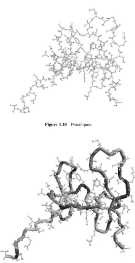
Figure 1.10 shows procolipase, as extracted from the Brookhaven PDB. The PDB serial number is 1PCN, and the molecule contains some 700 atoms.

Hydrogen atoms were not determined in the experimental studies, but most packages have an option to add hydrogen atoms. Protein structures can be complex and difﬁcult to interpret. For that reason, workers in the ﬁeld have developed alter-native methods of rendering these molecules. The idea is to identify the structural backbone of the molecule. To do this, we identify the backbone of each amino acid, and these are linked together as Figure 1.11 shows.

This particular rendering is thetube representation. Again, the use of colour makes for easier visualization, although this is lost in the monochrome illustrations given here.

(31)

[image:31.476.100.375.48.583.2]

Figure 1.10 Procolipase

Figure 1.11 Procolipase tube representation PROTEINS

(32)

(33)

2

Electric Charges

and Their Properties

As far as we can tell, there are four fundamental types of interactions between physical objects. There is the weak nuclear interaction that governs the decay of beta particles, and the strong nuclear interaction that is responsible for binding together the particles in a nucleus. The familiargravitational interaction holds the earth very ﬁrmly in its orbit round the sun, and ﬁnally we know that there is an

electromagneticinteraction that is responsible for binding atomic electrons to nuclei

and for holding atoms together when they combine to form molecules.

Of the four, the gravitational interaction is the only one we would normally come across in our everyday world. This is because gravitational interactions between bodies always add. The gravitational interaction between two atoms is negligible, but when large numbers of fundamental particles such as atoms are aggregated together, the gravitational interaction becomes signiﬁcant.

You may think it bizarre that there are four types of interaction, yet on the other hand you might wonder why there should be just four. Why not one, three or ﬁve? Should there not be a unifying theory to explain why there are four, and whether they are related? As I write, there is no such unifying theory despite tremendous research activity.

2.1 Point Charges

(34)

I’m sure you know that the best known fundamental particles responsible for these charges are electrons and protons, and you are probably expecting me to tell you that the electrons are the negatively charged particles whilst protons are positively charged. It’s actually just a convention that we take, we could just as well have called electrons positive.

Whilst on the subject, it is fascinating to note that the charge on the electron is exactly equal and opposite of that on a proton. Atoms and molecules generally contain exactly the same number of electrons and protons, and so the net charge on a molecule is almost always zero. Ions certainly exist in solutions of electrolytes, but the number of Naþ ions in a solution of sodium chloride is exactly equal to the number of Cl ions and once again we are rarely aware of any imbalance of charge.

A thunderstorm results when nature separates out positive and negative charges on a macroscopic scale. It is thought that friction between moving masses of air and water vapour detaches electrons from some molecules and attaches them to others. This results in parts of clouds being left with an excess of charge, often with specta-cular results. It was investigations into such atmospheric phenomena that gave the ﬁrst clues about the nature of the electrostatic force.

We normally start any study of charges at rest (electrostatics) by considering the force between two point charges, as shown in Figure 2.1.

The term ‘point charge’ is a mathematical abstraction; obviously electrons and protons have a ﬁnite size. Just bear with me for a few pages, and accept that a point charge is one whose dimensions are small compared with the distance between them. An electron is large if you happen to be a nearby electron, but can normally be treated as a point charge if you happen to be a human being a metre away.

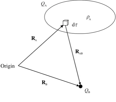
[image:34.476.155.318.465.610.2]

The concept of a point charge may strike you as an odd one, but once we have established the magnitude of the force between two such charges, we can deduce the force between any arbitrary charge distributions on the grounds that they are com-posed of a large number of point charges.

(35)

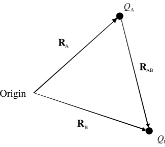
In Figure 2.1 we have point chargeQA at position vectorRA andQBat pointRB.

From the laws of vector analysis, the vector

RAB¼RB RA

joinsQAtoQB, and points fromQAtoQBas shown. I have indicated the direction of

the vectors with arrows.

2.2 Coulomb’s Law

In 1785, Charles Augustin de Coulomb became the ﬁrst person to give a mathema-tical form to the force between point charges. He measured the force directly between two very small charged bodies, and was able to show that the force exerted byQAon

QBwas

proportional to the inverse square of the distance betweenQAandQBwhen both

charges were ﬁxed;

proportional to QAwhen QBandRAB were ﬁxed; and

proportional to QBwhenQAandRABwere ﬁxed.

He also noticed that the force acted along the line joining the centres of the two charges, and that the force was either attractive or repulsive depending on whether the charges were different or of the same type. The sign of the product of the charges therefore determines the direction of the force.

A mathematical result of these observations can be written in scalar form as

FA on B/

QAQB

R2 AB

ð2:1Þ

Forces are vector quantities, and Equation (2.1) is better written in vector form as

FA on B /

QAQB

R3AB RAB

When Coulomb ﬁrst established his law, he had no way to quantify charge and so could not identify the proportionality constant. He took it to be unity, and thereby deﬁned charge in terms of the force between charges. Modern practice is to regard charge and force as independent quantities and because of this a dimensioned pro-portionality constant is necessary. For a reason that need not concern us, this is taken as 1=ð4E₀_{Þ, where the permittivity of free space}E₀_{is an experimentally determined}

COULOMB’S LAW

(36)

quantity with the approximate valueE₀_¼_8.854₁₀ 12_C2_N 1_m 2_{. Coulomb’s law}

is therefore

FA on B¼

1 4E₀

QAQB

R3_AB RAB ð2:2Þ

and it applies to measurements done in free space. If we repeat Coulomb’s experi-ments with the charges immersed in different media, then we ﬁnd that the law still holds but with a different proportionality constant. We modify the proportionality constant using a quantityE_rcalled therelative permittivity. In older texts,E_ris called

thedielectric constant. Our ﬁnal statement of Coulomb’s law is therefore

FA on B¼

1 4E_rE₀

QAQB

R3 AB

RAB ð2:3Þ

According to Newton’s Third Law, we know that ifQAexerts a forceFA on BonQB,

thenQBshould exert an equal and opposite force onQA. Coulomb’s law satisﬁes this

requirement, since

FB on A¼

1 4E_rE₀

QAQB

R3 BA

RBA

(the vectorRBApoints in the opposite direction toRABand so one force is exactly the

negative of the other, as it should be).

2.3 Pairwise Additivity

Suppose we now add a third point chargeQCwith position vector RC, as shown in

Figure 2.2. SinceQAand QBare point charges, the addition of QCcannot alter the

force betweenQA andQB.

(37)

The total force on QB now comprises two terms, namely the force due to point

chargeQA and the force due to point chargeQC. This total force is given by

FB ¼

QB

4E₀

QA

RAB

R3 AB

þQC

RCB

R3 CB

ð2:4Þ

This may seem at ﬁrst sight to be a trivial statement; surely all forces act this way. Not necessarily, for I have assumed that the addition ofQCdid not have any effect on

QA andQB(and so did not inﬂuence the force between them).

The generic term pairwise additive describes things such as forces that add as above. Forces between point electric charges are certainly pairwise additive, and so you might imagine that forces between atoms and molecules must therefore be pairwise additive, because atoms and molecules consist of (essentially) point charges. I’m afraid that nature is not so kind, and we will shortly meet situations where forces between the composites of electrons and protons that go to make up atoms and molecules are far from being pairwise additive.

2.4 The Electric Field

Suppose now we have a point chargeQat the coordinate origin, and we place another point chargeqat point P that has position vectorr(Figure 2.3). The force exerted by

Qonqis

F¼ 1 4E₀

Qq r3 r

which I can rewrite trivially as

F¼

1 4E₀

Q r3r

q

Figure 2.3 Field concept

THE ELECTRIC FIELD

(38)

The point is that the term in brackets is to do withQand the vectorr, and contains no mention ofq. If we want to ﬁnd the force on any arbitraryqatr, then we calculate the quantity in brackets once and then multiply byq. One way of thinking about this is to imagine that the chargeQcreates a certain ﬁeld at pointr, which determines the force on any otherqwhen placed at positionr.

This property is called theelectric fieldEat that point. It is a vector quantity, like force, and the relationship is that

Fðonqat rÞ ¼qEðat rÞ

Comparison with Coulomb’s law, Equation (2.3), shows that the electric ﬁeld at point

rdue to a point chargeQ at the coordinate origin is

E¼ 1 4E₀

Qr

r3 ð2:5Þ

E is sometimes written E(r) to emphasize that the electric ﬁeld depends on the position vectorr.

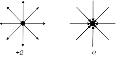
Electric fields are vector fields and they are often visualized asfield lines. These are drawn such that their spacing is inversely proportional to the strength of the field, and their tangent is in the direction of the field. They start at positive charges and end at negative charges, and two simple examples are shown in Figure 2.4. Here the choice of eight lines is quite arbitrary. Electric fields that don’t vary with time are called

electrostaticﬁelds.

2.5 Work

[image:38.476.140.336.64.166.2]

Look again at Figure 2.3, and suppose we move point chargeqwhilst keepingQﬁxed in position. When a force acts to make something move, energy is transferred. There is a useful word in physical science that is to do with the energy transferred, and it is work. Work measures the energy transferred in any change, and can be calculated from the change in energy of a body when it moves through a distance under the inﬂuence of a force.

(39)

We have to be careful to take account of the energy balance. If a body gains energy, then this energy has to come from somewhere, and that somewhere must lose energy. What we do is to divide the universe into two parts: the bits we are interested in called

thesystemand the rest of the universe that we call thesurroundings.

Some texts focus on the work done bythe system, and some concern themselves with the work doneonthe system. According to the Law of Conservation of Energy, one is exactly the equal and opposite of the other, but we have to be clear which is being discussed. I am going to write won for the work done on our system. If the

system gains energy, thenwonwill be positive. If the system loses energy, thenwon

will negative.

We also have to be careful about the phrase ‘through a distance’. The phrase means ‘through a distance that is the projection of the force vector on the displacement vector’, and you should instantly recognize a vector scalar product (see the Appendix). A useful formula that relates to the energy gained by a system (i.e. won) when a

constant forceFmoves its point of application throughlis

won¼ F l ð2:6Þ

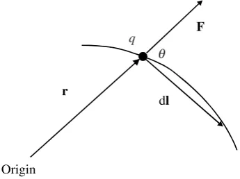
In the case where the force is not constant, we have to divide up the motion into differential elements dl, as illustrated in Figure 2.5. The energy transferred is then given by the sum of all the corresponding differential elements dwon. The

corre-sponding formulae are

dwon¼ F dl

won¼

Z

F dl ð2:7Þ

We now moveqby an inﬁnitesimal vector displacement dlas shown, so that it ends up at pointrþdl. The work done on the system in that differential change is

dwon¼ F dl

Figure 2.5 Electrostatic work

WORK

(40)

If the angle between the vectorsrI and dl is , then we have

dwon ¼ Fdlcos

and examination of Figure 2.6 shows that dlcos is the radial distance moved by chargeq, which we will write as dr. Hence

dwon¼

1 4E₀

Qq r2 dr

The total work done moving from position I to position II is therefore found by integrating

won¼

1 4E₀

Z II

I

Qq r2 dr

¼ 1

4E₀Qq

1 rII

1 rI

ð2:8Þ

The work done depends only on the initial and ﬁnal positions of the chargeq; it is independent of the way we make the change.

Another way to think about the problem is as follows. The force is radial, and we can divide the movement from position I to position II into inﬁnitesimal steps, some of which are parallel toFand some of which are perpendicular toF. The perpendi-cular steps count zero towardswon, the parallel steps only depend on the change in the

(scalar) radial distance.

2.6 Charge Distributions

[image:40.476.151.324.65.194.2]

So far I have concentrated on point charges, and carefully skirted round the question as to how we deal with continuous distributions of charge. Figure 2.7 shows a charge

(41)

distribution QA. The density of charge need not be constant through space, and we

normally write(r) for the density at the point whose position vector isr. The charge contained within the volume element d atris therefore(r) dand the relationship between(r) andQA is discussed in the Appendix. It is

QA¼

Z

ðrÞd ð2:9Þ

In order to ﬁnd the force between the charge distribution and the point chargeQBwe

simply extend our ideas about the force between two point charges; one of the point charges being(r) d and the otherQB.

The total force is given by the sum of all possible contributions from the elements of the continuous charge distributionQAwith point chargeQB. The practical

calcula-tion of such a force can be a nightmare, even for simple charge distribucalcula-tions. One of the reasons for the nightmare is that forces are vector quantities; we need to know about both their magnitude and their direction.

In the next section I am going to tell you about a very useful scalar field called the mutual potential energyU. This field has the great advantage that it is a scalar field, and so we don’t need to worry about direction in our calculations.

2.7 The Mutual Potential Energy

U

Suppose now we start with chargeqat inﬁnity, and move it up to a point with vector positionr, as shown in Figure 2.3. The work done is

won¼

1 4E₀

Qq

[image:41.476.144.334.65.231.2]

r ð2:10Þ

Figure 2.7 Charge distribution

THE MUTUAL POTENTIAL ENERGY

(42)

and this represents the energy change on building up the charge distribution, with the charges initially at inﬁnite separation. It turns out that this energy change is an important property, and we give it a special name (the mutual potential energy) and a special symbolU (occasionallyF_).

Comparison of the equations for force, work and mutual potential energy given above suggests that there might be a link between the force and the mutual potential energy; at ﬁrst sight, one expression looks like the derivative of the other. I am going to derive a relationship between force and mutual potential energy. The relationship is perfectly general; it applies to all forces provided that they are constant in time.

2.8 Relationship Between Force and Mutual

Potential Energy

Consider a body of massmthat moves in (say) thex-direction under the inﬂuence of a constant force. Suppose that at some instant its speed isv. The kinetic energy is1

2mv 2_.

You are probably aware of the law of conservation of energy, and know that when I add the potential energyU to the kinetic energy, I will get a constant energy"

"¼1 2mv

2_þ_U _ð2:11Þ

I want to show you how to relateUto the forceF. If the energy"is constant in time, then d"=dt¼0. Differentiation of Equation (2.11) with respect to time gives

d" dt ¼mv

dv dtþ

dU dt

and so, by the chain rule

d" dt ¼mv

dv dt þ

dU dx

dx dt

If the energy"is constant, then its ﬁrst differential with respect to time is zero, andv is just dx=dt. Likewise, dv=dt is the acceleration and so

0¼

md

2_x

dt2 þ

dU dx

dx

dt ð2:12Þ

Equation (2.12) is true if the speed is zero, or if the term in brackets is zero. Accord-ing to Newton’s second law of motion, mass times acceleration is force and so

F¼ dU

dx ð2:13Þ

(43)

When working in three dimensions, we have to be careful to distinguish between vectors and scalars. We treat a body of mass m whose position vector is r. The velocity is v¼dr=dt and the kinetic energy is1

2m(dr=dt) (dr=dt). Analysis along

the lines given above shows that the forceFandUare related by

F¼ gradU ð2:14Þ

where the gradient of U is discussed in the Appendix and is given in Cartesian coordinates by

gradU ¼@U @xexþ

@U @yeyþ

@U

@z ez ð2:15Þ

Hereex,ey andezare unit vectors pointing along the Cartesian axes.

2.9 Electric Multipoles

We can deﬁne exactly an array of point charges by listing the magnitudes of the charges, together with their position vectors. If we then wish to calculate (say) the force between one array of charges and another, we simply apply Coulomb’s law [Equation (2.3)] repeatedly to each pair of charges. Equation (2.3) is exact, and can be easily extended to cover the case of continuous charge distributions.

For many purposes it proves more proﬁtable to describe a charge distribution in terms of certain quantities called the electric moments. We can then discuss the interaction of one charge distribution with another in terms of the interactions be-tween the electric moments.

Consider ﬁrst a pair of equal and opposite point charges, þQand Q, separated by distanceR (Figure 2.8). This pair of charges usually is said to form anelectric

dipole of magnitude QR. In fact, electric dipoles are vector quantities and a more

rigorous deﬁnition is

p_e¼QR ð2:16Þ

where the vectorRpoints from the negative charge to the positive charge.

We sometimes have to concern ourselves with a more general deﬁnition, one relating to an arbitrary array of charges such as that shown in Figure 2.9. Here we have four point charges:Q1whose position vector isR1,Q2whose position vector is

R2,Q3whose position vector isR3, andQ4whose position vector isR4. We deﬁne the

electric dipole momentpe of these four charges as

p_e¼X

4

i¼1

QiRi

ELECTRIC MULTIPOLES

(44)

It is a vector quantity with x, y and z Cartesian components X

4

i¼1

Q_iXi, X4

i¼1

Q_iYi

andX

4

i¼1

Q_iZi. This is consistent with the elementary deﬁnition given above; in the case

of two equal and opposite charges, þQand Q, a distancedapart, the electric dipole moment has magnitudeQd and points from the negative charge to the positive. The generalization toncharges is obvious; we substitutenfor 4 in the above deﬁnition.

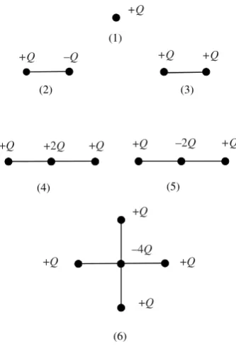
There are several general rules about electric moments of charge distributions, and we can learn a couple of the ones that apply to dipole moments by considering the simple arrays shown in Figure 2.10 and keeping the deﬁnitions in mind.

I have joined up the charges with lines in order to focus attention on the charge systems involved; there is no implication of a ‘bond’. We don’t normally discuss the electric dipole due to a point charge (1). Examination of the charge distributions (2)–(6) and calculation of their electric dipole moment for different coordinate origins suggests the general result; neutral arrays of point charges have a unique electric dipole moment that does not depend on where we take the coordinate origin. Otherwise, we have to state the coordinate origin when we discuss the electric dipole moment.

I can prove this from Equation (2.16), generalized to npoint charges

p_e¼X

n

i¼1

QiRi ð2:17Þ

Figure 2.8 Simple electric dipole

(45)

Suppose that we move the coordinate origin so that each point charge Qi has a

position vectorR0_i, where

Ri ¼R0iþ

witha constant vector. From the deﬁnition of the electric dipole moment we have

p_e¼X

n

i¼1

QiRi

and so, with respect to the new coordinate origin

p0_e¼X

n

i¼1

QiR0i

¼X

n

i¼1

QiðRi Þ

¼p_e X

n

i¼1

[image:45.476.155.322.61.306.2]

Qi

Figure 2.10 Simple arrays of point charges

ELECTRIC MULTIPOLES

(46)

The two deﬁnitions only give the same vector if the sum of charges is zero. We often use the phrasegauge invariantto describe quantities that don’t depend on the choice of coordinate origin.

Arrays (5) and (6) each have a centre of symmetry. There is a general result that any charge distribution having no overall charge but a centre of symmetry must have a zero dipole moment, and similar results follow for other highly symmetrical arrays of charges.

2.9.1 Continuous charge distributions

In order to extend the deﬁnition of an electric dipole to a continuous charge distribu-tion, such as that shown in Figure 2.7, we ﬁrst divide the region of space into differential elements d. If (r) is the charge density then the change in volume element d is(r)d. We then treat each of these volume elements as point charges and add (i.e. integrate). The electric dipole moment becomes

p_e¼

Z

rðrÞd ð2:18Þ

2.9.2 The electric second moment

The electric dipole moment of an array of point charges is deﬁned by the following three sums

Xn

i¼1

QiXi;

Xn

i¼1

QiYi and

Xn

i¼1

QiZi

and we can collect them into a column vector in an obvious way

p_e¼

Xn

i¼1

QiXi

Xn

i¼1

QiYi

Xn

i¼1

QiZi 0 B B B B B B B B @ 1 C C C C C C C C A ð2:19Þ

The six independent quantities X

n

i¼1

QiXi2, Xn

i¼1

QiXiYi, Xn

i¼1

QiXiZi;. . .; Xn

i¼1

QiZi2

(47)

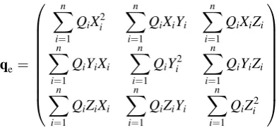
We usually collect them into a real symmetric 33 matrixqe

q_e¼

Xn

i¼1

QiX2i Xn

i¼1

QiXiYi Xn

i¼1

QiXiZi

Xn

i¼1

QiYiXi Xn

i¼1

QiYi2 Xn

i¼1

QiYiZi

Xn

i¼1

QiZiXi Xn

i¼1

QiZiYi Xn

i¼1

QiZi2 0 B B B B B B B B @ 1 C C C C C C C C A ð2:20Þ

The matrix is symmetric because of the obvious equalities of the off-diagonal sums such as

Xn

i¼1

QiXiYi and Xn

i¼1

QiYiXi

There are, unfortunately, many different deﬁnitions related to the second (and higher) moments in the literature. There is little uniformity of usage, and it is necessary to be crystal clear about the deﬁnition and choice of origin when dealing with these quantities.

Most authors prefer to work with a quantity called theelectric quadrupole moment rather than the second moment, but even then there are several different conventions. A common choice is to use the symbolQ_e _{and the deﬁnition}

Q_e_¼1

2

Xn

i¼1

Qið3Xi2 R 2 iÞ 3

Xn

i¼1

QiXiYi 3

Xn

i¼1

QiXiZi

3X

n

i¼1

QiYiXi

Xn

i¼1

Qið3Yi2 R 2 iÞ 3

Xn

i¼1

QiYiZi

3X

n

i¼1

QiZiXi 3

Xn

i¼1

QiZiYi

Xn

i¼1

Qið3Zi2 R 2 iÞ 0 B B B B B B B B @ 1 C C C C C C C C A ð2:21Þ

[image:47.476.140.338.82.174.2]

Note that the diagonal elements of this matrix sum to zero and so the matrix has zero trace (the trace being the sum of the diagonal elements, see the Appendix). Some authors don’t use a factor of 1₂ in their deﬁnition. Quadrupole moments are gauge invariant provided the electric dipole moment and the charge are both zero.

Figure 2.11 shows an octahedrally symmetrical array of point charges. Each point charge has magnitudeQ, apart from the central charge that has magnitude 6Qin order to make the system neutral. The distance between each axial point charge and the central one isa.

If I choose to direct the Cartesian axes along the symmetry axes, then the second moment matrix is

q_e¼Qa2

2 0 0

0 2 0

0 0 2

0

@

1

A

whilst the quadrupole moment matrix is zero.

ELECTRIC MULTIPOLES

(48)

If I now reduce the symmetry of the charge distribution by placing charges 2Qalong the vertical axis (taken for the sake of argument as thex-axis) and 8Qat the centre (to keep the electrical balance), the second moment matrix becomes

q_e¼Qa2

4 0 0

0 2 0

0 0 2

0

@

1

A

whilst the quadrupole moment matrix is now

Q_e_¼_Qa2

2 0 0

0 1 0

0 0 1

0

@

1

A

The electric quadrupole moment measures deviations from spherical symmetry. It is zero when the charge distribution has spherical symmetry. It always has zero trace (because of the deﬁnition), but it isn’t always diagonal. Nevertheless, it can always be made diagonal by a rotation of the coordinate axes.

Finally, consider a linear array formed by the top (þQ), central (þ2Q) and lower charges ( 3Q). We ﬁnd

q_e¼Qa2

2 0 0

0 0 0

0

@

1

A; Qe¼Qa2

2 0 0

0 1 0

0 0 1

0

@

1

A

In cases where the symmetry of the problem determines that the second moment tensor only has one non-zero component, we speak colloquially ofthe second mo-ment (which in this case is 2Qa2).

(49)

2.9.3 Higher electric moments

The set of 10 independent quantitiesX

n

i¼1

QiX3i, Xn

i¼1

QiX2iYi through Xn

i¼1

QiZ3i deﬁnes

the electric third moment of the charge distribution, and so on. We rarely encounter such higher moments of electric charge in chemistry.

2.10 The Electrostatic Potential

Electrostatic forces are vector quantities, and we have to worry about their magnitude and direction. I explained earlier that it is more usual to work with the mutual potential energy U rather than the force F, if only because U is a scalar quantity. In any case we can recover one from the other by the formula

F¼ gradU

Similar considerations apply when dealing with electrostatic fields. They are vector fields with all the inherent problems of having to deal with both a magnitude and a direction. It is usual to work with a scalar field called theelectrostatic potential. This is related to the electrostatic fieldE in the same way thatU is related toF

E¼ grad

We will hear more about the electrostatic potential in later sections. In the meantime, I will tell you that the electrostatic potential at ﬁeld pointrdue to a point chargeQat the coordinate origin is

ðrÞ ¼ Q 4E₀

1

r ð2:22Þ

The electric ﬁeld and the electrostatic potential due to an electric dipole, quadrupole and higher electric moments are discussed in all elementary electromagnetism texts. The expressions can be written exactly in terms of the various distances and charges involved. For many applications, including our own, it is worthwhile examining the mathematical form of these ﬁelds for points in space that are far away from the charge distribution. We then refer to (for example) the ‘small’ electric dipole and so on.

The electrostatic potential at ﬁeld pointr due to a small electric dipolepe at the

coordinate origin turns out to be

ðrÞ ¼ 1 4E₀

p_e r

r3 ð2:23Þ

which falls off as 1=r2. It falls off faster withrthan the potential due to a point charge because of the cancellation due to plus and minus charges. This is in fact a general

THE ELECTROSTATIC POTENTIAL

(50)

rule, the electrostatic potential for a small electric multipole of order l falls off as r (lþ1)so dipole moment potentials fall off faster than those due to point charges, and so on.

2.11 Polarization and Polarizability

In electrical circuits, charges are stored in capacitors, which at their simplest consist of a pair of conductors carrying equal and opposite charges. Michael Faraday (1837) made a great discovery when he observed that ﬁlling the space between the plates of a parallel plate capacitor with substances such as mica increased their ability to store charge. The multiplicative factor is called the relative permittivity and is given a symbol E_r_{, as discussed above. I also told you that the older name is the dielectric}

constant.

Materials such as glass and mica differ from substances such as copper wire in that they have few conduction electrons and so make poor conductors of electric current. We call materials such as glass and micadielectrics, to distinguish them from me-tallic conductors.

Figure 2.12 shows a two-dimensional picture of a dielectric material, illustrated as positively charged nuclei each surrounded by a localized electron cloud. We now apply an electrostatic ﬁeld, directed from left to right. There is a force on each charge, and the positive charges are displaced to the right whilst the negative charges move a corresponding distance to the left, as shown in Figure 2.13.

The macroscopic theory of this phenomenon is referred to asdielectric

polariza-tion, and we focus on the induced dipole moment dpe per differential volume d.

Because it is a macroscopic theory, no attention is paid to atomic details; we assume that there are a large number of atoms or molecules within the volume element d(or that the effects caused by the discrete particles has somehow been averaged out).

(51)

We relate the induced electric dipole to the volume of a differential element by

dp_e¼Pd ð2:24Þ

where the dielectric polarizationPis an experimentally determined quantity. Pcan depend on the applied ﬁeld in all manner of complicated ways, but for very simple media and for low ﬁeld strengths, it turns out thatPis directly proportional toE. We write