10 (2000) 91 – 106
The use of domestic and world market indexes
in the estimation of time-varying betas
Michael D. McKenzie *, Robert D. Brooks, Robert W. Faff
School of Economics and Finance,Royal Melbourne Institute of Technology,GPO Box2476V,
Melbourne,Vic.3001,Australia
Received 28 January 1998; accepted 25 February 1999
Abstract
This paper generates time-varying estimates of Australian industry betas relative to an Australian market index and a world market index using the Kalman filter approach. As a means of comparison, these conditional estimated betas are used to forecast each industry’s return in-sample. The forecast error metrics suggest that the estimates of conditional risk relative to the domestic market index are preferred to estimates generated using the world market index, irrespective of the industry concerned. While not to suggest time-varying betas estimated relative to a domestic index are universally superior, these results suggest that they are preferable in certain circumstances. © 2000 Elsevier Science B.V. All rights reserved.
Keywords:Time-varying beta; Market index; Kalman filter
JEL classification:G12
www.elsevier.com/locate/econbase
1. Introduction
There is growing evidence which suggests that the world’s capital markets are
generally becoming more integrated1
. In the Australian context, Ragunathan et al.
* Corresponding author. Tel.: +61-3-9925-5891; fax:+61-3-9925-5986.
E-mail addresses: michael [email protected] (M.D. McKenzie), [email protected] (R.D. Brooks), [email protected] (R.W. Faff)
1These studies include: (a) CAPM framework — Stehle (1977); Errunza and Losq (1985); Jorion and Schwartz (1986); Errunza et al. (1992) and Bekaert and Harvey (1995); (b) APT framework — Cho et al. (1986) and Gultekin et al. (1989); (c) CAPM/APT — Korajczyk and Viallet (1989) and Mittoo (1992); and (d) Consumption CAPM framework — Wheatley (1988). The interested reader is referred to Naranjo and Protopapadakis (1997) (p. 95, Table 1) who provide a useful comparative table of recent integration studies and Alford (1993) for a good textual summary of many of these papers.
M.D.McKenzie et al./J.of Multi.Fin.Manag.10 (2000) 91 – 106 92
(1999) use a CAPM framework to assess the extent of integration of the Australian market over the period 1974 – 1992 taking into account (1) business cycles (Aus-tralian and US); and (2) deregulation of the Aus(Aus-tralian financial markets. The pre-deregulation period is taken to end in November 1983, prior to the floating of the Australian dollar in the following month. While their findings are somewhat mixed, their general conclusion is that the market is segmented prior to
deregula-tion and integrated in the post-dereguladeregula-tion period2.
In the case where a country’s capital market is integrated into world markets, the appropriate benchmark becomes a world (rather than a domestic) market portfolio in an asset pricing context. As such, risk should be measured against a world market index rather than a domestic country index. A variation of this argument centres on differences in industrial structure. Specifically, where a commodity is traded between nations and its price is determined in the interna-tional market place, global factors may be argued to dominate over domestic factors in determining the returns of companies operating in such a market. In this case, the more appropriate index against which risk should be measured may be a world market index, rather than the domestic market index. This argument is potentially most relevant to the resources sector as Grinold et al. (1989) (p. 87) for example, have argued that most ‘‘…global industries appear to be related to fungible commodities such as money, oil, chemicals and precious metals’’.
Given the results of Ragunathan et al. (1999) for the Australian market, how do we expect the domestic and international betas to perform against one another in capturing risk over a similar sample period? In particular, will estimates of beta generated relative to the domestic index be inferior in the post-deregula-tion period where the results generally favoured the integrapost-deregula-tion hypothesis? While the answer to this question seems obvious, it need not be so as although integrated markets seemingly compel the use of an international market bench-mark, it may turn out that beta estimated relative to the domestic index is adequate.
The primary focus of the current paper is to investigate the relative superiority of beta risk measured against a domestic and a world market index. In light of the
considerable evidence that beta risk is not constant3, this paper will investigate
conditional betas based on a Kalman filtering approach. Further, the observation
that integration may vary by industry motivates the use of industry portfolios4. The
remainder of this paper is structured as follows. In Section 2 we present the
2They also concluded that business cycles had a role to play. Specifically, it seemed more likely that markets are integrated (segmented) in expansionary (contractionary) phases of business cycles.
3Evidence may be found in Fabozzi and Francis (1978); Bos and Newbold (1984); Collins et al. (1987); Faff et al. (1992); Brooks et al. (1992, 1994); Wells (1994); Bos and Fetherston (1995); Pope and Warrington (1996); Cheng (1997).
methodology by which unconditional betas may be estimated and com-pared. Section 3 details the data to be analysed in this study and presents some descriptive statistics. Time-varying betas are then generated for this data and the results are discussed in Section 4. Finally, Section 5 presents a summary and conclusions.
2. Method of analysis
A number of different techniques exist by which one may estimate time-varying betas: the multivariate generalised ARCH (M-GARCH) model first introduced by Bollerslev (1990); a time-varying beta market model approach suggested by Schwert and Seguin (1990); and the Kalman filter approach. All three of these approaches to generating time-varying beta have each been applied independently in a variety of contexts5.
Recently, Brooks et al. (1998a) compared each of these three techniques against one another, using a common dataset of Australian industry portfolios over the period 1974 – 1996. Brooks et al. generated results which overwhelm-ingly supported the Kalman filter approach as the optimal technique by which to generated time-varying betas. A limitation of that paper however, was that it reported results of conditional betas estimated relative to a domestic market index only. As discussed earlier, the evidence suggests that in the post-deregulation period (after November 1983), it is likely that the Australian market was largely integrated. Consequently, the current paper seeks to extend the analysis contained in Brooks et al. (1998a) to investigate the relative performance of conditional betas using both a domestic and a world market index. Based on the apparent superiority of the Kalman filter approach reported by Brooks et al. in the Australian context, we adopt this method to generate estimates of conditional beta.
In previous research, the Kalman filter approach has been used by Black et al. (1992) and Wells (1994). Black et al. (1992) examined the performance of a sample of 30 UK unit trusts over the 1980s. Regarding the issue of unstable risk, they found that for all but three of their funds, the time series properties indicated time-varying betas over their sample period. Wells (1994) investigated the time series properties of beta risk for a sample of 10 stocks listed on the Stockholm exchange over the period 1971 – 1989. His results also support a conclusion of time-varying beta for the majority of his sample and interestingly that the random walk model is preferred.
The Kalman filter approach to estimating time-varying beta (bit) involves a
measurement Eq. (1); transition Eqs. (2a) and (2b); and prior conditions (Eq. (3)) as follows:
M.D.McKenzie et al./J.of Multi.Fin.Manag.10 (2000) 91 – 106 94
Rit=at+bitRMt+ot otN(0, V) (1)
where:
at=at−1+ut utN(0, Q1) (2a)
bt=bt−1+ht htN(0, Q2) (2b)
given the prior:
b0N(b0,P0) (3)
where Rit is the return for asset i in period t and RMt is the return on either the
domestic market or world market index. This technique recursively estimates the
entire series providing conditional estimates of both bit and ait.
To provide one view of whether the domestic or world market index performs
better as a conditional beta risk benchmark, an in-sample forecast (Rˆit) comparison
is applied. Specifically, a Kalman filter-based forecast return may be generated as:
Rˆit=ait+bitRMt (4)
where bit and ait are produced by the Kalman filter approach applied to both the
world and domestic market index.
Following Brooks et al. (1998a), we assess the accuracy of the forecasts using the mean absolute forecasting error (MAE) and the mean square forecasting error
(MSE)6. The MAE is calculated as:
MAEi=% T
t=1
Rˆit−Rit/T (5)
Alternatively, the MSE is calculated as:
MSEi= %
T
t=1
(Rˆit−Rit)
2
/T (6)
Thus, the MAE and MSE measures of forecasting error will be used to compare the performance of the conditional beta series estimated relative to a world and domestic market index.
3. Data
Our data are monthly adjusted price relative information for 24 Australian Stock Exchange (ASX) industries taken from the Price Relatives File of the Centre for Research in Finance (CRIF) at the Australian Graduate School of Management (details of these industries are provided in the tables). Our full sample period extends from January 1974 to May 1995. Two alternative proxies are used for the
market portfolio, namely, a value-weighted domestic market index supplied by the CRIF and a value-weighted global market index supplied by Morgan Stanley. All data were expressed in Australian dollars and continuously compounded percentage returns were created for the analysis.
A summary of the descriptive statistics for these industry returns data may be found in Brooks et al. (1998a) and, hence, are not reported here. When comparing the return of the domestic market index to that of the world market index, it was found that the mean return on the Australian index is higher than that of the world index (0.116 and 0.0099, respectively) and the S.D. is larger (0.0598 and 0.0418).
Further, the domestic and world index are both negatively skewed (−2.5056 and
−0.4569), exhibit severe kurtosis (22.887 and 4.945) and fail the test of normality
(Jacque Bera values of 4679.3 and 49.8, respectively). In each of these comparisons, the return on the world index is more normally behaved than its domestic counterpart. This observation, in part, reflects the fact that the October 1987 stock
market crash was much more severe in Australia than it was globally7.
4. Empirical results
The standard market model was estimated for each of the Australian industry portfolios, firstly using the domestic index as the market proxy. The results are presented in the second column of Table 1 and reveal that each of the beta estimates are significantly different from zero and with the exception of the Developers and Contractors; Transport; and Media industries, different from unity. The market model was then re-estimated using the world market index as the benchmark and the results are also presented in Table 1, column 3. Examining these results one can see that using the world index in comparison to the domestic index generates (numerically) considerably lower risk estimates in each instance. The highest beta in this case was only 0.793 for the Entrepreneurial Investors category which is significantly lower than (1) the counterpart beta of 1.206 relative to the domestic market index and (2) the highest beta value across all industries of 1.356 estimated for the Gold industry against the domestic index. At the other end of the spectrum, the lowest world beta value of 0.246 for the Property Trusts industry was much lower than the counterpart beta of 0.434 estimated relative to the domestic market index. Each of the betas generated against the world market index was significantly different from zero and significantly less than unity.
The evidence provided by the literature suggests that these market model parameters are likely to be unstable over time. Indeed, the tests of parameter stability applied to these data confirm this general finding. Specifically, in the case where the domestic market index is used as the relevant benchmark, the cumulative sum of squares (CUSUMSQ) test of Brown et al. (1975) suggests beta parameter instability for 20 of the 24 industries. Fig. 1 presents a graphical result of the
7Indeed, the Australian market monthly return on the CRIF value weighted index was approximately
M
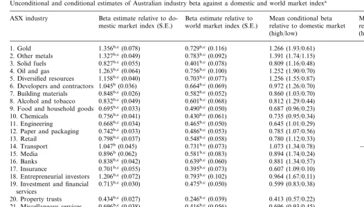
Unconditional and conditional estimates of Australian industry beta against a domestic and world market indexa Mean conditional beta
Beta estimate relative to do- Beta estimate relative to Mean conditional beta ASX industry
relative to domestic market
mestic market index (S.E.) world market index (S.E.) relative to World Market (high/low) (high/low)
0.575 (1.62/−0.14) 0.729b,c(0.116)
1. Gold 1.356b,c(0.078) 1.266 (1.93/0.61)
1.327b,c(0.049)
2. Other metals 0.783b,c(0.092) 1.391 (1.74/1.15) 0.733 (1.51/0.17) 0.827b,c(0.055) 0.401b,c(0.078) 0.809 (1.16/0.48) 0.323 (0.79/−0.11) 3. Solid fuels
0.715 (1.61/0.22) 4. Oil and gas 1.263b,c(0.064) 0.756b,c(0.100) 1.252 (1.90/0.70)
0.659 (1.17/0.05) 5. Diversified resources 1.158b,c(0.040) 0.703b,c(0.077) 1.256 (1.55/0.87)
0.972 (1.26/0.70) 0.504 (1.26/0.04) 6. Developers and contractors 1.045b(0.036) 0.664b,c(0.069)
0.848b,c(0.026) 0.582b,c(0.052) 0.860 (1.03/0.70) 0.505 (0.93/0.20) 7. Building materials
0.508 (1.23/0.20) 8. Alcohol and tobacco 0.832b,c(0.049) 0.601b,c(0.068) 0.812 (1.29/0.44)
0.695b,c(0.033) 0.490b,c(0.050) 0.687 (0.96/0.23) 0.414 (0.91/0.11) 9. Food and household goods
10. Chemicals 0.756b,c(0.041) 0.430b,c(0.061) 0.735 (0.95/0.34) 0.329 (0.84/0.03) 0.668b,c(0.034) 0.465b,c(0.050) 0.645 (1.01/0.29) 0.368 (0.80/0.10) 11. Engineering
0.742b,c(0.033) 0.486b,c(0.053) 0.785 (1.07/0.56)
12. Paper and packaging 0.436 (0.92/0.18)
0.105 (0.73/−0.37) 13. Retail 0.798b,c(0.037) 0.548b,c(0.058) 0.780 (1.12/0.33)
1.047b(0.045) 0.731b,c(0.073) 1.073 (1.34/0.78) −0.018 (0.33/−0.30) 16. Banks 0.838b,c(0.042)
0.101 (0.41/−0.21) 17. Insurance 0.701b,c(0.055) 0.395b,c(0.073) 0.607 (1.09/0.10)
18. Entrepreneurial investors 1.206b,c(0.072) 0.793b,c(0.102) 0.964 (1.67/0.11) 0.178 (0.53/−0.19) 0.029 (0.26/−0.31) 0.713b,c(0.030) 0.475b,c(0.050) 0.599 (0.83/0.38)
19. Investment and financial services
0.434b,c(0.027) 0.246b,c(0.039) 0.413 (0.57/0.22) 0.087 (0.46/−0.44) 20. Property trusts
21. Miscellaneous services 0.696b,c(0.038) 0.416b,c(0.056) 0.696 (0.93/0.45) 0.122 (0.48/−0.29) 0.664b,c(0.031) 0.424b,c(0.049) 0.592 (0.86/0.39) 0.292 (0.65/−0.34) 24. Tourism and leisure 0.509b,c(0.045)
0.964
r(bi,bit) – – 0.489
aThis table presents the standard market model point estimates of beta generated relative to a domestic Australian market index as well as relative to a world market index. The mean conditional beta estimated using the Kalman filter approach relative to the domestic market index and the world index is presented in the final two columns with the range of beta observations in parentheses.
CUSUMSQ test for a representative case, namely, the Property Trust industry. In this figure, it can be seen that the plot of the recursive residuals first breaches the 5% boundary in approximately late 1975 indicating a shift in regime. The four exceptions which did not exhibit such parameter instability were the Building Materials, Chemicals, Retail and Diversified Industrials sectors. Fig. 2 presents a
Fig. 1. The CUSUMSQ test of beta stability in the market model equation for the Australian property trusts industry. The recursive residuals exceed the 5% bound of significance indicating instability of the beta parameter in the market model regression using the domestic market index. This result was also found for 19 other industries tested.
M.D.McKenzie et al./J.of Multi.Fin.Manag.10 (2000) 91 – 106 98
plot of the CUSUMSQ test for the Chemicals industry which is representative of these cases.
The CUSUMSQ test results for the market model estimated using the world market index as the benchmark indicate that the finding of widespread beta instability is not contingent on the index used. That is, the test results in this case show that for all 24 industries, the recursively estimated residuals exceeded the 5% critical boundary.
Given the evidence of beta instability discussed above, it is appropriate to analyse time-varying beta risk. To this end, the Kalman filter model was used to generate conditional beta risk estimates for the 24 industries relative to both the domestic
market index and the world index8,9
. The final two columns of Table 1 present the mean value of beta generated relative to both the domestic and world index, as well as the range of beta observations (in parentheses). Table 1 reveals that the mean of
thebitseries generated for the domestic index, provides a similar measure of risk to
the standard market model — the cross-sectional correlation between the beta estimate and the mean Kalman beta is 0.964. The largest range of observations generated by the Kalman approach was evidenced in the Entrepreneurial Investors
sector (1.67/0.11), while the smallest range of observations was found in the
Building Materials sector (1.03/0.70).
The final column of Table 1 presents the mean beta value and the range of beta observations for the conditional beta series generated relative to the world market. The highest mean value of conditional beta was 0.733 in the Other Metals industry,
while the lowest mean value was −0.18 for the Transport industry. Examining the
range of these betas relative to the world index, one can observe that even excluding the first 2 years of data, negative minimum beta values are commonly observed. The highest range of observations for conditional beta was found in the Gold
industry (1.62/ −0.14), while the smallest range was found in the Investment and
Financial Services industry (0.26/ −0.31).
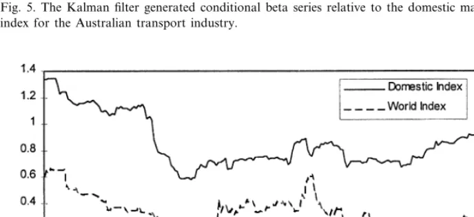
Figs. 3 – 6 present plots of the conditional beta series generated using the Kalman filter method relative to both the world market index and the domestic market
index10. As can be seen in these figures, the world market index generally produced
lower estimates of industry risk and this was a common feature across all industries. Further we observe that for some industries, conditional beta increased significantly at the time of the 1987 crash (such as for the Gold and Alcohol and Tobacco
8Estimates of conditional beta were also generated using the M-GARCH and Schwert and Seguin approach referred to in Section 2 and in-sample forecasts of the industry return generated. These results are qualitatively similar to the Kalman approach and so are not presented in this paper to conserve space. However, they are available from the authors upon request.
9The Kalman filter approach is prone to a ‘start-up’ value problem, namely, that very large (and in some cases negative) parameter values are often generated in the initial stages of estimation. We avoid this problem by excluding the first 2 years of observations from the remainder of the analysis leaving a restricted sample commencing in January 1976.
Fig. 3. The Kalman filter generated conditional beta series relative to the domestic market and world index for the Australian gold industry.
Fig. 4. The Kalman filter generated conditional beta series relative to the domestic market and world index for the Australian alcohol and tobacco industry.
M.D.McKenzie et al./J.of Multi.Fin.Manag.10 (2000) 91 – 106 100
obtained by considering the correlation between each series over the entire sample
period11. Further, we also allow for possible changes in correlation between various
subperiods where the break point relates to possible structural changes in the Australian economy. Harper and Scheit (1992) suggest that for the Australian economy a pre-deregulatory subperiod may be defined which ends in November 1983, just prior to the floating of the Australian dollar in December of that year.
Fig. 5. The Kalman filter generated conditional beta series relative to the domestic market and world index for the Australian transport industry.
Fig. 6. The Kalman filter generated conditional beta series relative to the domestic market and world index for the Australian banking industry.
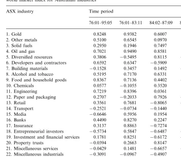
Table 2
Correlation between the Kalman filter generated conditional beta estimated relative to a domestic and world market index for Australian industriesa
ASX industry Time period
3. Solid fuels 0.2950 0.1946
0.8581 0.6538 0.9490
4. Oil and gas 0.7021
0.3806 −0.5495 0.8115 −0.1155 5. Diversified resources
−0.5909 0.5661 0.6347
6. Developers and contractors 0.6592
0.1492 −0.5870 7. Building materials −0.1528 0.3457
0.6331 0.7296 0.7170
8. Alcohol and tobacco 0.5195
0.4402 −0.3179 9. Food and household goods 0.8367 0.7136
0.3520 0.6397 12. Paper and packaging 0.2707
0.7681
0.3561 −0.8065 −0.4343
13. Retail 19. Investment and financial services
0.8147 0.7036 20. Property trusts −0.0394 0.2663
−0.6657 −0.4737 0.1481
21. Miscellaneous services −0.0429
−0.3091 −0.0967 −0.4907 0.1640
0.3735 −0.1441 −0.3814
24. Tourism and leisure
0.0677 0.2088 0.4509
0.2446 Average
aThe table presents the correlation coefficient for the conditional beta series generated by the Kalman filter method using both a domestic Australian market index and a world market index over the entire sample period and also in subperiods. To prevent a ‘start-up’ bias, the first 2 years of data were excluded.
The second subperiod suggested by Harper and Scheit (1992) covers the period February 1984 to September 1987 which ends just prior to the stock market crash of October 1987. Finally, a third subperiod for analysis covers the period Novem-ber 1987 to the end of our full sample period in May 1995.
correla-M.D.McKenzie et al./J.of Multi.Fin.Manag.10 (2000) 91 – 106 102
tion for the Gold industry was also very high (0.82). However, such high correla-tions tended not to be the norm. Indeed, for seven industries, a negative correlation
coefficient was generated, with the lowest case of −0.66 for the Media industry.
The average correlation coefficient across all twenty-four industries tested was 0.24 which indicates that on average, these two conditional beta series possess dissimilar patterns over time.
Examining the correlation coefficients in each of the subperiods defined, one finds a rather interesting result. In the pre-deregulatory subperiod (1976:01 – 1983:11) the average correlation coefficient was 0.45, with only five industries revealing a negative association (most of these were close to zero). However, after the floating of the Australian dollar in December 1983, the correlation between the conditional beta series generated using the world and the domestic market index decreases quite markedly. Specifically, the average correlation drops to a low 0.06 and the number of industries exhibiting a negative correlation increases from five to 10 (42% of the sample). Further, when we consider the third and final subperiod the correlations tend to rise again. Indeed, the average conditional beta correlation increases to 0.20 and, although the number of negative coefficients does not change markedly (nine in all), they are generally closer to zero. The gold industry provides a good illustrative example. In the pre-deregulatory period the correlation between the conditional gold betas was 0.93. It then dropped to 0.60 following the float of the dollar but in the period after the stock market crash, the correlation had again risen to 0.93. This pattern is typical for about a third of the industries under study. This would appear to indicate that any changes to the relationship between the returns of an industry and the domestic and world market index introduced by the floating
of the dollar were transitory12.
From the above discussion, it is apparent that differences exist between the bit
series generated using each of the world and domestic market index. This suggests that the results of any study containing estimates of conditional beta may in part be influenced by the index against which market risk is assessed. As such, it is worthwhile comparing the ‘performance’ of beta estimates produced by the domes-tic and world market index. As outlined in the previous section we will do this by
forecasting each industry return series in-sample (Rˆit) and then compare the
forecast error produced in terms of the MAE and MSE metrics. The results of this procedure are presented in Table 3.
A comparison of the forecasts generated using the world market index to the forecasts based on betas measured against the domestic market index, reveals considerable support for the domestic market beta approach. Specifically, the data
presented in Table 3, show that theRˆitbased on the domestic country index are more
‘accurate’ in comparison to the forecasts generated using the world market index in each instance. This is reflected in the lower average MAE obtained when using the domestic conditional betas (0.0184) compared to the case using international
Table 3
MAE and MSE forecast error resultsa
ASX industry MAE MSE
Domestic market
Domestic market World market World market index
2. Other metals 0.00043 0.00142
0.00042 0.00067 0.0204
3. Solid fuels 0.0158
0.0272
0.0175 0.00057
4. Oil and gas 0.00126
0.00024 0.00087 5. Diversified resources 0.0120 0.0230
0.00064 6. Developers and contrac- 0.0113 0.0191 0.00020
tors
0.00041 0.00012
7. Building materials 0.0090 0.0164 0.138
8. Alcohol and tobacco 0.0186 0.00040 0.00067
0.00018
18. Entrepreneurial in- 0.0209 0.0674 0.00077 0.01100 vestors
0.00410 19. Investment and financial0.0087 0.0415 0.00014
services
0.0083 0.00339
20. Property trusts 0.0403 0.00011
21. Miscellaneous services 0.0121 0.0474 0.00028 0.00388 0.00324 22. Miscellaneous industri- 0.0095 0.0428 0.00015
als
0.00408 23. Diversified industrials 0.0090 0.0462 0.00013
0.0145 0.0473 0.00035 0.00366
24. Tourism and leisure
0.0184 0.0362 0.00319
Average 0.00033
M.D.McKenzie et al./J.of Multi.Fin.Manag.10 (2000) 91 – 106 104
conditional betas (0.0362). The MSE, which places a heavier penalty on outliers, reinforces this result as again for each of the 24 industries the domestic model generates a lower MSE and in some cases the difference is quite marked. One example, is the Entrepreneurial Investors industry where the domestic model provided an MSE of 0.00077 compared to an MSE value of 0.0110 for its international counterpart. The average MSE across all industries reflected the general superiority of the domestic market based conditional betas as the average MSE was considerably lower (0.00033) compared to the average MSE for the conditional betas relative to the world index (0.00319).
Given that conditional betas estimated relative to a domestic market index generate more accurate forecasts of returns in-sample, can we say that time-varying betas based on a domestic index are preferred to those based on an international index? The answer to this question must be considered carefully and is not immediately obvious. For example, the answer may depend on whether we take an asset pricing perspective or a hedging perspective. From an asset pricing point of view, the answer depends on whether the integration hypothesis holds. In seg-mented markets, the risk premia attaches to the domestic beta and it is the relevant risk measure. However, when markets are integrated the risk premia relates to the international beta and it becomes the relevant risk measure. These issues are not the focus of the current paper as they have been addressed elsewhere (Ragunathan et al., 1999). Consequently, our analysis does not say anything about whether the market is integrated or not. Alternatively, if we take the view of a mutual fund manager interested in hedging, even in the case of integrated markets or integrated industries, the results of this paper find support for the use of a domestic index benchmark against which to estimate conditional beta risk. For example, a mutual fund manager trying to hedge should be using domestic index futures contracts
because the domestic index has a higher correlation with all industries13
.
5. Summary and conclusions
The appropriate choice of index against which to measure beta risk is an important empirical question. Accordingly, this paper compared Kalman filter estimates of conditional beta generated using a domestic Australian market index and a world market index. Based on the comparison of in-sample forecast errors, the estimates of conditional risk relative to the domestic market index were preferred to estimates generated using the world market index. However, while our findings favour domestic time-varying betas over their international counterparts, this is not to suggest that their superiority is universal. Indeed, from an asset pricing point of view, the integrated property of modern capital markets suggests the use of a global market benchmark. Further, for industries that are integrated (primarily because their commodity prices are determined in the international market place),
risk should again be measured against a world market index. However, if we take the view of a mutual fund manager interested in hedging, even in the case of integrated markets, our findings provide support for the domestic index benchmark.
Acknowledgements
The authors wish to thank an anonymous referee for his helpful comments on an earlier version of this paper.
References
Alford, A., 1993. Assessing capital market segmentation: A review of the literature. In: Stansell, S. (Ed.), International Financial Market Integration. Blackwell, Oxford.
Ball, R., Brown, P., 1980. Risk and return from equity investments in the Australian mining industry: January 1958 – February 1979. Aust. J. Manage. 5, 45 – 66.
Bekaert, G., Harvey, C.R., 1995. Time-varying world market integration. J. Finance 50, 403 – 444. Black, A., Fraser, P., Power, D., 1992. UK unit trust performance 1980 – 1989: A passive time varying
approach. J. Banking Finance 16, 1015 – 1033.
Bollerslev, T., 1990. Modelling the coherence in short run nominal exchange rates: A multivariate generalised ARCH model. Rev. Econ. Stat. 72, 498 – 505.
Bos, T., Fetherston, T.A., 1995. Nonstationarity of the market model, outliers, and the choice of market rate of return. In: Bos, T., Fetherston, T.A. (Eds.), Advances in Pacific-Basin Financial Markets 1. JAI Press.
Bos, T., Newbold, P., 1984. An empirical investigation of the possibility of systematic stochastic risk in the market model. J. Bus. 57, 35 – 41.
Braun, P., Nelson, D., Sunier, A., 1995. Good news, bad news, volatility and betas. J. Finance 50 (5), 1575 – 1603.
Brooks, R.D., Faff, R.W., Lee, J.H.H., 1992. The form of time variation of systematic risk: Some Australian evidence. Appl. Financial Econ. 2, 191 – 198.
Brooks, R.D., Faff, R.W., Lee, J.H.H., 1994. Beta stability and portfolio formation. Pacific-Basin Finance J. 2, 463 – 479.
Brooks, R.D., Faff, R.W., McKenzie, M.D., 1998a. Time varying beta risk of Australian industry portfolios: A comparison of modelling techniques. Aust. J. Manage. 23, 1 – 22.
Brooks, R., Faff, R., Ho, Y.K., McKenzie, M.D., 1998b. U.S. banking sector risk in an era of regulatory change: A bivariate GARCH approach. Review of Quantitative Finance and Accounting, in press.
Brown, R., Durbin, J., Evans, J.M., 1975. Techniques for testing the constancy of regression relation-ships over time. J. R. Stat. Soc. 37, 145 – 164.
Cheng, J.W., 1997. A switching regression approach to the stationality of systematic and non-systematic risks: the Hong Kong experience. Appl. Financial Econ. 7 (1), 45 – 58.
Cho, D., Eun, C., Senbet, L., 1986. International arbitrage pricing theory: An empirical investigation. J. Finance 41, 313 – 330.
Collins, D.W., Ledolter, J., Rayburn, J., 1987. Some further evidence on the stochastic properties of systematic risk. J. Bus. 60, 425 – 448.
Episcopos, A., 1996. Stock return volatility and time varying betas in the Toronto stock exchange. Q. J. Bus. Econ. 35, 28 – 38.
M.D.McKenzie et al./J.of Multi.Fin.Manag.10 (2000) 91 – 106 106
Errunza, V., Losq, E., Padmanabhan, P., 1992. Tests of integration, mild segmentation and segmenta-tion hypotheses. J. Banking Finance 16, 949 – 972.
Fabozzi, F.J., Francis, J.C., 1978. Beta as a random coefficient. J. Financial Quant. Anal. 13, 101 – 115. Faff, R.W., Lee, J.H.H., Fry, T.R.L., 1992. Time stationarity of systematic risk: Some Australian
evidence. J. Bus. Finance Accounting 19, 253 – 270.
Giannopoulos, K., 1995. Estimating the time varying components of international stock markets’ risk. Eur. J. Finance 1, 129 – 164.
Gonzalez-Rivera, G., 1996. Time varying risk: The case of the American computer industry. J. Empir. Finance 2, 333 – 342.
Grinold, R., Rudd, A., Stefek, D., 1989. Global factors: Fact or fiction? J. Portfolio Manage., Fall, pp. 79 – 88.
Gultekin, M.N., Gultekin, N.B., Penati, A., 1989. Capital controls and international capital market segmentation: The evidence from the Japanese and American stock markets. J. Finance 44, 849 – 869. Harper, I., Scheit, T., 1992. The effects of financial market deregulation on bank risk and profitability.
Aust. Econ. Pap. 31, 260 – 271.
Jorion, P., Schwartz, E., 1986. Integration versus segmentation in the Canadian stock market. J. Finance 41, 603 – 613.
Korajczyk, R., Viallet, C., 1989. An empirical investigation of international asset pricing. Rev. Financial Stud. 2, 553 – 587.
Koutmos, G., Lee, U., Theodossiou, P., 1994. Time varying betas and volatility persistence in international stock markets. J. Econ. Bus. 46, 101 – 112.
McClain, K.T., Humphreys, H.B., Boscan, A., 1996. Measuring risk in the mining sector with ARCH models with important observations on sample size. J. Empir. Finance 3, 369 – 391.
Mittoo, U., 1992. Additional evidence on integration in the Canadian stock market. J. Finance 47, 2035 – 2054.
Naranjo, A., Protopapadakis, A., 1997. Financial market integration tests: An investigation using US equity markets. J. Int. Financial Markets Inst. Money 7, 93 – 135.
Pope, P., Warrington, M., 1996. Time-varying properties of the market model coefficients. Accounting Res. J. 9 (2), 5 – 20.
Ragunathan, V., Brooks, R., Faff, R., 1999. Correlations, business cycles and integration, Journal of International Financial Markets, Institutions and Money 9, 75 – 95.
Schwert, G.W., Seguin, P.J., 1990. Heteroscedasticity in stock returns. J. Finance 4, 1129 – 1155. Stehle, R., 1977. An empirical test of the alternative hypotheses of national and international pricing of
risky assets. J. Finance 32, 493 – 502.
Wells, C., 1994. Variable betas on the Stockholm exchange 1971 – 1989. Appl. Econ. 4, 75 – 92. Wheatley, S., 1988. Some tests of international equity integration. J. Financial Econ. 21, 177 – 212.