Income Inequality, and Mortality
Ulf-G. Gerdtham
Magnus Johannesson
a b s t r a c t
We test whether mortality is related to individual income, mean commu-nity income, and commucommu-nity income inequality, controlling for initial health status and personal characteristics. The analysis is based on a ran-dom sample from the adult Swedish population of more than 40,000 indi-viduals who were followed up for 10– 17 years. We nd that mortality de-creases signicantly as individual income inde-creases. For mean community income and community income inequality we cannot, however, reject the null hypothesis of no effect on mortality. This result is stable with respect to a number of measurement and specication issues explored in an exten-sive sensitivity analysis.
I. Introduction
Many studies have shown a positive association between income and survival (see, for instance, the overview of results in Viscusi 1994 and Lutter and Morrall 1994). This is consistent with the view that an increase in income increases investments in health-enhancing goods, and that health is a normal good (Grossman 1972). However, it has also been argued that it is an individual’s relative rather than absolute income that is important for health, with a low relative income being a health hazard (Marmot et al. 1991; Wilkinson 1997, 1998). A low relative income could, for instance, be associated with increased psychosocial stress leading to dis-ease (Cohen, Tyrrell, and Smith 1991; Cohen et al. 1997). In conjunction with the
Ulf-G Gerdtham is a professor of Community Medicine at Lund University, Sweden. Magnus Johannes-son is a professor of Economics at the Stockholm School of Economics. The authors thank Bjo¨rn Lindgren, Katarina Steen Carlsson, and an anonymous referee for helpful comments and suggestions. The data used in this article can be obtained beginning August 2004 through July 2007 from Ulf-G Gerdtham, Department of Community Medicine, Lund University, Malmo¨ University Hospital, SE-205 02 Malmo¨, Sweden. E-mail: ulf.gerdtham” smi.mas.lu.se.
[Submitted March 2001; accepted July 2002]
ISSN 022-166Xã2004 by the Board of Regents of the University of Wisconsin System
Gerdtham and Johannesson 229
relative-income hypothesis, it has furthermore been suggested that income inequality may be a health hazard in itself (Wilkinson 1996). From a policy perspective it is essential to be able to discriminate between these three hypotheses: the absolute-income hypothesis, the relative-absolute-income hypothesis, and the absolute-income-inequality hypothesis. If it is relative rather than absolute income that affects health, a doubling of everyone’s income would, for example, have no effect on health.
The income-inequality hypothesis has been supported by international comparison data showing a strong correlation between income inequality and mortality after controlling for the average income (Rodgers 1979; Flegg 1982; Waldmann 1992; Wilkinson 1996). However, as noted by for instance Smith (1999), it is very difcult to make empirical distinctions between the effects of income and income inequality using aggregate data. This is because a nonlinear concave relationship between in-come and life-expectancy at the individual level will generate a negative relationship between income inequality and life-expectancy at the aggregate level (controlling for the average income). Hence such a relationship cannot per se be interpreted as evidence that income inequality is a health hazard.
To differentiate between the different income hypotheses, individual-level data should ideally be used (Wagstaff and Van Doorslaer 2000; Gravelle, Wildman, and Sutton 2000). Recently a number of studies using individual level data have also been published in the public health eld, testing the income-inequality hypothesis on the state or county level in the United States.1These studies can be divided into
studies on assessed health status and studies on mortality. The studies on self-assessed health status have tended to nd an adverse effect of income inequality on health status (Soobader and LeClere 1999; LeClere and Soobader 2000; Kennedy et al. 1998; Kahn et al. 2000). Two exceptions to this result are the studies by Shibuya, Hashimoto, and Yano (2002) and Sturm and Gresenz (2002) that nd no signicant effect after controlling for individual characteristics. The results for mortality are mixed. Fiscella and Franks (1997, 2000), Daly et al. (1998), and Osler et al. (2002) nd no signicant effect of income inequality on mortality, whereas Lochner et al. (2001) nd a signicantly hazardous effect of income inequality on mortality. The studies by Fiscella and Franks (1997, 2000) and Daly et al. (1998) are based on relatively small samples yielding limited statistical power. The study by Lochner et al. (2001) is based on a large sample size, but do not control for mean community income and potentially important covariates like education. The study by Osler et al. (2002) only investigates small areas of residence (parishes) within a single city (Copenhagen in Denmark).
The studies in the public health eld have generated a lot of interest also among economists (Deaton 1999, 2001; Deaton and Paxson 1999; Meara 1999; Miller and Paxson 2000; Mellor and Milyo 2001, 2002). For the present study the contributions by Meara (1999) and Mellor and Milyo (2002) are particularly interesting since they use a similar methodology. Both studies use individual level data to test the effect of state level income inequality on health, infant health (low birth weight) in the Meara (1999) study, and self-assessed health status in the Mellor and Milyo (2002) study. Neither of the studies nds a signicant effect of income inequality on health status.
The present paper extends previous work on the effects of income and income inequality on health in several respects. In contrast to Meara (1999) and Mellor and Milyo (2002) we use mortality as the health measure. We are also the rst study to explicitly discriminate between the absolute-income hypothesis, the relative-income hypothesis, and the income-inequality hypothesis in the same study.2Our study is
based on high-quality register data on both disposable income and mortality, whereas most previous studies are based on self-reported categorical income measures (see the overview by Deaton 2001). We also use a large data set with more than 40,000 individuals followed up for 10–17 years, and we control more comprehensibly for individual characteristics than in most previous studies (age, gender, education, unem-ployment, immigration, urbanization, marital status, the number of children, and ini-tial health status). To nd the optimal functional relationship between income and the mortality rate, we use a Box-Cox analysis. In an extensive sensitivity analysis we also explore a number of measurement and specication issues. Our main nding is that individual income has a protective effect on mortality consistent with the abso-lute-income hypothesis, whereas for the relative-income hypothesis and the income-inequality hypothesis we cannot reject the null hypothesis of no effect on mortality. While we think our analysis and data offers many advantages compared to previ-ous studies, there are also some important limitations. One limitation is that Sweden, given its reputation as an egalitarian country, may not be the best laboratory for studying the inuence of income inequality on health. To be able to detect an effect of income inequality on mortality across geographical regions it is necessary to have sufcient variation in income inequality across regions. Both the level of income inequality and the variations may be important. The level of income inequality is clearly lower in Sweden than in the United States (Bishop, Formby, and Smith 1991). The variation in income inequality across municipalities in our data (the Gini coef-cient varies between 0.12 and 0.51), however, seem to be similar to that in the U.S. studies, at least compared to the variation between states in the United States (Fis-cella and Franks 1997; Daly et al. 1998; Meara 1999; Soobader and LeClere 1999; LeClere and Soobader 2000; Kahn et al. 2000; Lochner et al. 2001; Mellor and Milyo 2002). A further potential problem with Sweden is that the measured income inequality in Sweden may overstate true income inequality given the public services available in Sweden (that are not included in measured income). It is, however, not obvious that the omission of public consumption introduces more bias in income inequality in Sweden than in the United States. On the one hand the share of public consumption is higher in Sweden than in the United States (OECD 1998). On the other hand public consumption may be more targeted towards low-income groups in the United States. Nearly all health care in Sweden is for instance provided within the public health care system (even for high income groups), whereas in the United States the public nancing is targeted towards the poor (Medicaid) and the elderly (Medicare). Another limitation is that we have assumed that relative income and income inequality are important on the community level, and we may not have
Gerdtham and Johannesson 231
ned the appropriate “community.” It may also be the relative income and income inequality for the country rather than the community that is important for health, and this cannot be tested with our data. Furthermore, the relevant reference group to dene relative income may not be individuals who live in the same area; the relevant reference group could well be dened with respect to some other dimension like occupation or education (Deaton and Paxson 1999).
The paper is organized as follows. In the next section the data and methods used are outlined. A results section and an extensive sensitivity analysis follow this. The paper ends with some concluding remarks.
II. Data and methods
To test the absolute-income hypothesis, the relative-income hypothe-sis, and the income-inequality hypothesis we estimate the mortality risk as a function of individual income, mean community income, and community income inequality. In these estimations we also control for initial health status (the health status at the start of follow-up) and a number of exogenous personal characteristics that may be related to the mortality risk.3Relative income can be dened as the income of an
individual relative to the mean income of a reference group (Deaton 1999; Deaton and Paxson 1999). It is not obvious what constitutes the relevant reference group of individuals. The present paper is based on the presumption that the relevant reference group consists of individuals who live in the same area (Miller and Paxson 2000; Fiscella and Franks 1997; Daly et al. 1998). Even with this denition, the geographical area that encompasses a reference group remains to be specied. In U.S. studies it has been common to use the state as the reference group (Daly et al. 1998; Meara 1999; Miller and Paxson 2000; Mellor and Milyo 2002). In the baseline analysis we use municipalities as the reference group. Sweden consisted of 284 municipalities during the time of this study (with populations from about 3,000 to about 700,000). We use the same data set as employed by Gerdtham and Johannesson (2002) in their recent estimation of the income loss that will induce a fatality. The data set is based on Statistic Sweden’s Survey of Living Conditions (the ULF survey) (Statistics Sweden 1997), which has been linked to all-cause mortality data from the National Causes of Death Statistics (which registers all deaths of individuals registered as living in Sweden) and to income data from the National Income Tax Statistics. Since 1975, Statistics Sweden conducts annual surveys of living conditions in the form of one-hour personal interviews with randomly selected adults aged 16–84 years. In this paper we use pooled data from the interviews conducted in 1980– 86 for all the subjects aged 20–84 years at the time of the interview. The total sample consists of 43,898 individuals. After correcting for missing values, the sample is reduced to 41,006 individuals. In Table 1 the variables in the regression analysis are supplied and summary statistics are given.
T
h
e
Journal
of
H
um
an
R
es
ourc
es
Table 1
Descriptive statistics of the variables used in the regression analysis. Number of observations541,006
Standard
Variable Mean deviation Minimum Maximum
Dependent variable
Survival timea 12.549 3.330 0.0027397 16.86895
Survival status (51 if dead at the end of follow-up) 0.164 0.370 0 1 Independent variables, individual level
Annual disposable incomeb 106,820 44,497 1 2,778,470
Annuity of net wealthb 12,856 38,409 1 5,327,592
Annual incomeb,c 119,676 64,375 2 8,106,061
No limitations in functional abilityd
Some limitations in functional ability 0.086 0.281 0 1 Severe limitations in functional ability 0.092 0.290 0 1 Self-assessed health status: poor healthd
Self-assessed health status: fair health 0.190 0.392 0 1 Self-assessed health status: good health 0.750 0.433 0 1
High blood pressure 0.081 0.272 0 1
Male 0.496 0.500 0 1
Age 46.657 17.116 20 84
No children in the householdd
One child in the household 0.150 0.357 0 1
Two children in the household 0.159 0.366 0 1
G
erdtham
and
Johanne
ss
on
233
Nonimmigrantd
First generation immigrante 0.080 0.271 0 1
Second generation immigrantf 0.007 0.086 0 1
Single (not married or cohabiting) 0.310 0.463 0 1 Presecondary educationd
Short secondary education (#2 years) 0.309 0.462 0 1 Secondary education (.2 years) 0.096 0.295 0 1
University education 0.180 0.384 0 1
Unemployed 0.024 0.152 0 1
Included in the study 1980d
Included in the study 1981 0.145 0.353 0 1
Included in the study 1982 0.162 0.368 0 1
Included in the study 1983 0.147 0.355 0 1
Included in the study 1984 0.160 0.366 0 1
Included in the study 1985 0.146 0.353 0 1
Included in the study 1986 0.105 0.307 0 1
Independent variables, aggregate levelg
Mean income of the municipality 116,655 12,833 93,084 230,963 Gini coefcient of the municipality 0.183 0.032 0.117 0.511 Urbanization (inhabitants / km2in the municipality) 118.9225 378.4317 0 3,537
a. The number of life-years from inclusion in the study to the end of follow-up.
b. Per adult person in the household in 1996 Swedish Crowns (SEK; exchange rate 1996 $15SEK 6.71, purchasing power parity 1996 $15SEK 9.83). c. Annual income5annual disposable income1annuity of net wealth.
d. Baseline category in the regression analysis.
A. Dependent variable
The dependent variable in the regression analysis is the survival time in years and the survival status at the end of the follow-up period. The date of death was recorded for all subjects who had died by December 31, 1996. The survival time is estimated as the number of years from the interview date to the date of death. The censored survival time of persons alive at the end of 1996 is estimated as the number of years from the interview date to December 31, 1996.
B. Independent variables
1. Individual income
Our income measure consists of two components that are added together: annual disposable income and the annuity of net wealth. In our data set we have information about the disposable income of the household in the interview year. Disposable in-come consists of inin-come from capital (interest rates, dividends, and capital gains), income from employment and business and all income transfers (for example pension payments, unemployment benets, paid sick leave, housing assistance) net of taxes. Disposable income is converted to 1996 prices using the consumer price index.4The
disposable income of the household is divided by two for persons who are married or cohabiting, in order to obtain the disposable income per adult person in the house-hold. From the National Income Tax Statistics we also have information about the taxable net wealth (total taxable assets minus total liabilities) of the household during the interview year, which is converted to the net wealth at market value (see Gerd-tham and Johannesson 2002 for the details of this estimation). The net wealth of the household is converted to 1996 prices using the consumer price index and is divided by two for persons who are married or cohabiting, in order to obtain the net wealth per adult person in the household. The annuity of net wealth is based on the life-expectancy for men and women of different ages in Sweden and a 3 percent interest rate (Statistics Sweden 1998).
2. Community income and income inequality
We estimate the mean income in each municipality from our data, and this variable is included to test the relative-income hypothesis. The mean annual income varies between about 93,000 and SEK 231,000 in the different municipalities. The relative-income hypothesis implies that mortality should increase with mean community in-come, holding individual income constant. The coefcient of community income should also be of the same size (but with the opposite sign) as individual income if mortality is solely determined by relative income (this implies that a doubling of everyone’s income leaves mortality unchanged). In our baseline analysis we use the Gini coefcient as the measure of income inequality, but in a sensitivity analysis we also use a number of other measures of income inequality. The Gini coefcient is estimated for each municipality based on our data and varies between about 0.12
Gerdtham and Johannesson 235
and about 0.51 in the different municipalities. The income-inequality hypothesis im-plies that mortality should increase with the Gini coefcient.
3. Initial health status
We include three different variables for initial health status from the ULF survey: self-assessed health status (poor health, fair health, good health), functional ability [no limitations in functional ability, some limitations in functional ability (unable to run a short distance but able to climb stairs without difculty), severe limitations in functional ability (unable to run a short distance and unable to climb stairs without difculty)], and high blood pressure (persons diagnosed with hypertension). 4. Additional independent variables
We include the following personal characteristics: age, gender, immigration, unem-ployment, education, marital status, and the number of children. To control for any differences in health risks and costs of living between more and less populated areas we include a variable for urbanization (the number of inhabitants per square kilome-ter in the municipality of the individual). Finally, we include six dummy variables for the year of inclusion into the study, to control for any differences between the populations included in different years.
C. Estimation methods
To estimate the effect of income and the other covariates on the mortality risk, we estimate a Cox proportional hazard model (Cox 1972).5Standard errors are estimated
taking a possible intracluster correlation within Swedish municipalities into account.6
All variables except age, urbanization, individual income, mean community income, and community income inequality are entered as dummy variables. Age is included without any transformation, which implies an exponential relationship between age and mortality risk.7As individual income can be expected to be most important at
low income levels, a highly nonlinear relationship between individual income and mortality is expected. We use the same functional form for individual income and community income, to be able to compare the size of the coefcients directly. To nd the optimal functional relationship between income and the mortality rate, a Box-Cox analysis is carried out (Box and Cox 1964); that is, we estimate the optimal Box-Cox transformation parameterq as dened by the operator:X(q)5(Xq
21) /q
for q ¹0 or ln Xforq 50, whereXis income. A one-dimensional grid search is carried out over the interval21 to 1 for qat increments of 0.01 to determine the maximum likelihood point estimate forq. The Gini coefcient and the urbanization variable are entered untransformed. All tests of statistical signicance are carried out on the 5 percent level.
5. We also use a probit model as well as some common parametric duration models (the Weibull, exponen-tial, log-normal, gamma and Gompertz models) (Greene 1997). These models lead to similar results as the Cox model and do not change the reported conclusions below.
6. Estimation was undertaken using the cluster option in STATA, with the municipalities serving as the clustering variable.
7. We also test including a dummy variable for each age in the data, but this does not signicantly improve the model according to a likelihood ratio test (criticalc2
582.49; computedc2
III. Results
A. Baseline results
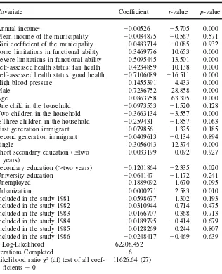
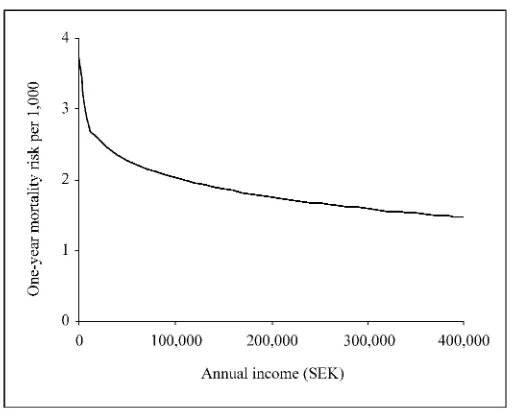
The results of the estimated Cox model are shown in Table 2. Individual income is highly signicant with a negative sign, implying that the mortality risk decreases with higher income. The log-likelihood function is maximized with a Box-Cox trans-formation parameter for income of 0.31 (q50.31). This functional form of income is signicantly different from both untransformed income (criticalc2
53.84; com-putedc2
514.94) and the logarithm of income (criticalc2
53.84; computedc2
5
15.12).8The relationship between annual income and the one-year mortality risk is
shown in Figure 1. As can be seen in the gure, the relationship is highly nonlinear with a decreasing effect of income at higher income levels. The community income variable has a negative sign, contrary to the relative-income hypothesis. The variable is, however, far from signicant. The community Gini coefcient also has a negative sign, and it is nonsignicant. We cannot therefore reject the null hypothesis that mortality is unaffected by relative income and income inequality at the municipality level.
B. Sensitivity analysis
The results of a number of sensitivity analyses are shown in Table 3. The income measure is varied in the sensitivity analysis. We rst reestimate our results without including the annuity of net wealth in our income measure. This leads to similar results as for the baseline analysis. We also reestimate our results with household income and household income per adult equivalent instead of household income per adult person in the household.9In these estimations income is signicant with
the expected negative sign, whereas the mean community income and the Gini coef-cient are not signicant. We also reestimate our results excluding individuals be-low 25 years of age and 30 years of age respectively, because many younger individ-uals may be college students with a current income that is a poor prediction of life-time income. This has little effect on the results. In another analysis, we exclude all individuals below 65 years of age (the retirement age in Sweden). For the remaining persons the annual income may be expected to be very stable over time, since their main source of income consists of pension payments that are stable over time. This reduces the estimated income coefcient slightly from 20.0053 to 20.0042, but the coefcient is still highly signicant. We also reestimate our results with two alternative functional forms of income and mean community income (the loga-rithm of income and untransformed income). This leads to qualitatively similar
8. We also test if the annual disposable income and the annuity of net wealth can be added together as one income measure, by testing if they differ signicantly if entered as separate variables. The estimated coefcients for annual disposable income and the annuity of net wealth are:20.0033 (t-value5 22.81) and20.0029 (t-value5 25.98). According to a Wald test we cannot reject the null hypothesis of the same effect of annual disposable income and the annuity of net wealth (criticalc2
53.84; computedc2
50.08).
Gerdtham and Johannesson 237
Table 2
Results from the Cox model (t-values adjusted for clustering on municipalities). Number of observations 541,006
Covariate Coefcient t-value p-value
Annual incomea
20.00526 25.705 0.000 Mean income of the municipality 20.0034875 20.567 0.571 Gini coefcient of the municipality 20.0483714 20.085 0.932 Some limitations in functional ability 0.3469776 10.653 0.000 Severe limitations in functional ability 0.5095445 13.501 0.000 Self-assessed health status: fair health 20.4234859 210.138 0.000 Self-assessed health status: good health 20.7106089 216.511 0.000
High blood pressure 0.1455391 4.433 0.000
Male 0.7236752 28.858 0.000
Age 0.0863758 63.305 0.000
One child in the household 20.0973553 21.520 0.128 Two children in the household 20.3663134 23.557 0.000
$Three children in the household 20.259431 21.857 0.063 First generation immigrant 20.079856 21.325 0.185 Second generation immigrant 20.0409613 20.134 0.894
Single 0.3056043 12.374 0.000
Short secondary education (#two 0.0033199 0.092 0.927 years)
Secondary education (.two years) 20.1201864 22.335 0.020
University education 20.064147 21.172 0.241
Unemployed 0.1889092 1.670 0.095
Urbanization 0.0000271 2.583 0.010
Included in the study 1981 0.0598677 1.302 0.193
Included in the study 1982 0.0310944 0.714 0.475
Included in the study 1983 0.0166707 0.368 0.713
Included in the study 1984 20.0189795 20.414 0.679
Included in the study 1985 0.0128269 0.244 0.807
Included in the study 1986 20.0248417 20.469 0.639
2Log-Likelihood 262208.452
Iterations Completed 6
Likelihood ratioc2(df) test of all coef- 11626.64 (27)
cients 50
a. The functional form of annual income is: (annual income0.31
Figure 1
The relationship between annual income and mortality (at the mean of the covari-ates).
results as in the baseline analysis, although the signicance of income decreases somewhat.
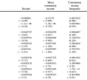
It has been argued that an increased income only decreases the mortality for individuals living in absolute or relative poverty (see Wagstaff and Van Doorslaer 2000) for an overview of this argument). To test this hypothesis, we reestimate our results excluding individuals at low-income levels (the 5 percent, 10 percent, 15 percent, and 20 percent poorest individuals are excluded in four analyses). The protective effect of individual income, however, remains after the poorest individuals have been excluded. We also test the sensitivity toward using other measures of income inequality than the Gini coefcient. We reestimate our results using the Robin Hood index (Kennedy, Kawachi, and Prothrow-Stith 1996), the income share of the 50 percent poorest individuals (Fiscella and Franks 1997), the variance of income, the variance of the logarithm of income (Deaton and Paxson 1999), and the coefcient of variation in income. Our results are, however, not sensitive toward the inequality measure used, and all inequality measures are far from being signicant.
G
erdtham
and
Johanne
ss
on
239
Table 3
Sensitivity analysis of the estimated coefcients of income, mean community income and community income inequality (t-values in parentheses adjusted for clustering on municipalities)
Mean Community community income Income income Inequality
Baseline result 20.00526 20.0034875 20.0483714
(25.705) (20.567) (20.085)
Alternative income measures
Annual household income per adult in the household (annuity of 20.0043982 20.003129 20.0743207
net wealth excluded) (23.770) (20.612) (20.117)
Annual household income (annuity of net wealth included) 20.0044667 20.002399 20.0211131
(25.374) (20.694) (20.040)
Annual household income (annuity of net wealth excluded) 20.0032678 20.0029827 20.0518246
(23.088) (20.812) (20.077)
Annual household income per adult equivalent (annuity of net 20.0054154 0.0034549 20.6283268
wealth included) (25.829) (0.535) (20.971)
Annual household income per adult equivalent (annuity of net 20.0046664 0.0020426 20.6532173
wealth excluded) (23.864) (0.366) (21.000)
Excluding different ages
Age,25 years excluded 20.005317 20.0037042 0.0093508
(25.701) (20.688) (0.015)
Age,30 years excluded 20.0051683 20.0033038 0.0045067
(25.505) (20.612) (0.007)
Age,65 years excluded 20.0041956 20.003627 20.3754456
T
h
e
Journal
of
H
um
an
R
es
ourc
es
Table 3(continued)
Mean Community community income Income income Inequality
Alternative functional form of income
Natural log of income 20.086886 20.23178 0.0033822
(24.499) (20.996) (0.006)
Untransformed income 21.11e206 21.34e206 0.0448461
(23.424) (20.729) (0.076)
Excluding the poorest individuals
5 percent poorest individuals excluded 20.0043757 20.0034076 0.0866697
(23.867) (20.637) (0.169)
10 percent poorest individuals excluded 20.0038701 20.0054668 0.1302324
(22.878) (20.985) (0.245)
15 percent poorest individuals excluded 20.0028343 20.0071051 0.2864644
(22.197) (21.186) (0.498)
20 percent poorest individuals excluded 20.003126 20.0079587 0.7532521
(22.211) (21.261) (1.165)
Alternative income inequality measures
Robin Hood index 20.0052556 20.0037275 0.0001582
(25.717) (20.605) (0.021)
Income share of the 50 percent poorest individuals 20.0052435 20.0043013 0.2894068
(25.71) (20.72) (20.29)
Variance of income 20.0052641 20.0031045 21.57e213
(25.725) (20.517) (20.647)
Variance of the logarithm of income 20.0052564 20.0036523 20.0019681
G
erdtham
and
Johanne
ss
on
241
Coefcient of variation of income 20.005266 20.0029746 24.31e208
(25.725) (20.491) (20.720)
Excluding small municipalities
Municipalities with,25 observations excluded 20.005241 20.0028319 20.1355153
(25.692) (20.528) (20.269)
Municipalities with,50 observations excluded 20.0054727 20.0054534 20.1652021
(25.770) (20.960) (20.302)
Municipalities with,75 observations excluded 20.0048806 20.0094775 0.2153093
(24.980) (21.309) (0.333)
Municipalities with,100 observations excluded 20.0052863 20.0080869 0.345395
(25.171) (21.006) (0.352)
Instrumental variable estimation
Split sample IV method for community variables and no instru- 20.0052793 20.0042037 0.3221342
mentation of individual income (25.724) (20.536) (0.209)
Split sample IV method for community variables and instru- 20.0060935 20.0085242 20.2694503
mented individual income (22.108) (21.084) (20.173)
Instrumented individual income and no instrumentation of com- 20.0059758 20.003973 21.30256
munity variables (22.073) (20.904) (20.874)
Alternative community denitions
Counties instead of municipalities 20.0050677 20.0523183 3.078016
(25.332) (22.327) (1.113)
Local labor markets instead of municipalities 20.0052411 20.010286 0.32479
(25.917) (21.221) (0.289)
Geographical xed effects
Local labor markets 20.0052413 0.0019028 20.0837946
(25.66) (0.22) (20.12)
Counties 20.0052042 0.0105819 20.3681249
(25.65) (1.58) (20.65)
Excluding regressor variables
Blood pressure excluded 20.0052277 20.0035334 20.0498471
T
h
e
Journal
of
H
um
an
R
es
ourc
es
Table 3(continued)
Mean Community community income Income income Inequality
All initial health status variables excluded 20.0084508 20.0021933 20.2401227
(29.60) (20.39) (20.39)
Education excluded 20.0056178 20.0039845 20.0729435
(26.30) (20.65) (20.13)
Annual income excluded — 20.0079185 0.1039548
(21.30) (0.18)
Annual income and health status variables excluded — 20.0092584 20.0155515
(21.66) (20.03)
Excluding subsamples
1980 subsample excluded 20.0056811 0.0009165 20.5299988
(25.939) (0.162) (20.964)
1981 subsample excluded 20.0051142 20.0009353 20.0547607
(25.416) (20.168) (20.097)
1982 subsample excluded 20.0049527 20.0017518 20.1801989
(24.801) (20.323) (20.317)
1983 subsample excluded 20.0056851 20.0053195 0.227986
(25.899) (20.894) (0.415)
1984 subsample excluded 20.0052763 20.000994 20.6854959
(25.078) (20.17) (21.116)
1985 subsample excluded 20.0049209 20.0045009 0.1403991
(24.74) (20.746) (0.263)
1986 subsample excluded 20.0054594 20.0025556 20.456
Gerdtham and Johannesson 243
with fewer than 25, 50, 75, and 100 observations.10The result for individual income
is almost identical to that of the baseline analysis in these sensitivity analyses and the mean community income and the Gini coefcient are not signicant in any of these analyses. We also use instrumental variables to try and correct for the potential measurement error problem. We use a split-sample instrumental variables technique, that is, we split the sample randomly into two parts of equal size and use estimates of the mean municipality income and the Gini coefcient from half the sample to instrument for the same variables computed from the other half of the sample (Miller and Paxson 2000). These sensitivity analyses lead to similar results as the baseline analysis. Also our measure of individual income could be subject to attenuation bias. It is based on disposable income in a single year and may be an imperfect measure of permanent income. Consequently, we carry out an instrumental variable estima-tion using the occupaestima-tional group of the individual and the number of rooms in the house / apartment of the individual as instruments. The instrumentation of income leads to a modest increase in the absolute size of the income coefcient, from about
20.0053 to about 20.0060. It also decreases the precision in the estimated coef-cient, but it is still signicant.
We also reestimate our results for two alternative geographical denitions of the community used to dene relative income and income inequality. In one analysis we use the county as the community. Sweden was divided into 24 counties at the time of this study and this represents a much greater degree of aggregation than municipalities. In another analysis we use local labor markets as the community. Sweden has been divided into 100 local labor markets by Statistics Sweden, and this level of aggregation represents an intermediate level between municipalities and counties. The alternative levels of aggregation lead to nearly identical results for the individual income variable. For local labor markets the community income variable is still negative, but not signicant. The coefcient for income inequality changes from a negative to a positive sign, but is still far from being signicant. The mean community income at the county level is negative and signicant. The negative sign is inconsistent with the relative-income hypothesis and suggests that the mean in-come of the county has a protective effect. The Gini coefcient at the county level has a positive sign, but it is not signicant. In another sensitivity analysis we test including additional controls for geographical areas. In one analysis we include xed effects for local labor markets and in one analysis we include xed county effects. This leads to nearly identical results for individual income. As before the mean community income and the Gini coefcient are not signicant, although the commu-nity income variable switches to a positive sign consistent with the relative-income hypothesis.
The sensitivity toward excluding different variables is also tested. Blood pressure may be related to lifestyle and is excluded. This has little effect on the results. In another analysis all variables for initial health status are excluded. This leads to a sizeable increase in the income coefcient to20.0085 (t-value5 29.60), but has little effect on the mean community income or income inequality variables. Exclud-ing education increases the income coefcient somewhat, but has little effect on the
other variables. We also test if the income inequality variable is affected by excluding income and excluding both income and initial health status, but this has little effect on the income inequality variable.11We also test the stability of the results by
exclud-ing each subsample from the estimations. The results are relatively stable towards the exclusion of any of the subsamples from the analysis. Mellor and Milyo (2002) also test what they refer to as the weak income-inequality hypothesis, that income inequality may affect only the least well off in society. We test this in a similar way to Mellor and Milyo (2002), by interacting the Gini coefcient with ve dummy variables for the ve income quintiles. None of these interaction coefcients are signicant. Finally we test for interaction effects between the three income measures and age and gender. The only signicant interaction is between age and income, suggesting that the income coefcient decreases with age.12The coefcients
andt-values for the mean community income and the community Gini coefcient are almost identical to the baseline model when the age and income interaction is included.
IV. Concluding Remarks
We have tried to discriminate between the absolute-income hypothe-sis, the relative-income hypothehypothe-sis, and the income-inequality hypothesis. According to our results, mortality decreased signicantly with individual income, controlling for mean community income and income inequality. The relationship between in-come and mortality was also, as expected, highly nonlinear with a decreasing effect of income at higher income levels. The protective effect of individual income was stable towards a large range of sensitivity analyses.
We found no signicant effect of community income inequality in our baseline analysis or in any of the sensitivity analyses. Generally speaking, we found no sig-nicant effect of mean community income on mortality either. The exception to this result arose when the community was dened on the county level rather than on the municipality level as in the baseline analysis. The mean county income was signi-cant with a negative sign, implying that a higher county mean income has a protective effect controlling for individual income. This is, however, contrary to the relative-income hypothesis. The coefcient for mean municipality relative-income in the baseline analysis had a negative sign, too, but was far from being signicant. It is not implau-sible that a high average community income could have a protective effect on health. Community income could, for instance, be associated with a number of factors with
Gerdtham and Johannesson 245
potential health effects, such as the provision of public goods, environmental quality, and access to health care (Miller and Paxson 2000).
Even when individual income was omitted from the regression community income inequality was not signicantly related to mortality. This is contrary to most individ-ual level studies for the United States, although also in the studies by Daly et al. (1998), Meara (1999), and Sturm and Gresenz (2002) community income inequality was not signicant when individual income was omitted (as long as other personal characteristics and community income was controlled for). This indicate that the consumption inequality may be much lower and less variable in Sweden than in the United States, and it is possible that this is the reason that we failed to nd a signi-cant association between income inequality and mortality in our analysis.
Overall our results are consistent with the absolute-income hypothesis, whereas we fail to conrm the relative-income hypothesis and the income-inequality hypothe-sis. Our results for mortality are consistent with the recent results of Meara (1999) and Mellor and Milyo (2002) for health status. However, further work is needed before the relative-income hypothesis and the income-inequality hypothesis can be rmly rejected.
References
Bishop, John, John Formby, and James Smith. 1991.“International Comparisons of Income Inequality: Tests for Lorenz Dominance across Nine Countries.” Economica58(232): 461– 77.
Box, G. E. P., and D. R. Cox. 1964. “An Analysis of Transformations.” Journal of the Royal Statistical Society, Series B 26(2):211– 43.
Chapman, Kenneth, and Govind Hariharan. 1994. “Controlling for Causality in the Link from Income to Mortality.”Journal of Risk and Uncertainty 8(1):85– 93.
Cohen, Sheldon, David Tyrrell, and Andrew Smith, 1991. “Psychological Stress and Sus-ceptibility to the Common Cold.”New England Journal of Medicine 325(9):606– 12.
Cohen, Sheldon, Scott Line, Stephen Manuck, Bruce Rabin, Eugene Heise, and Jay Kaplan. 1997. “Chronic Social Stress, Social Status, and Susceptibility to Upper Respira-tory Infections in Nonhuman Primates.”Psychosomatic Medicine59(3):213– 21.
Cox, D. R. 1972. “Regression Models and Life Tables.”Journal of the Royal Statistical So-ciety, Series B34(2):187– 220.
Daly, Mary, Greg Duncan, George Kaplan, and John Lynch. 1998. “Macro-to-Micro Links in the Relation between Income Inequality and Mortality.”Milbank Quarterly76(3): 315– 39.
Deaton, Angus. 1999. “Inequalities in Income and Inequalities in Health.” NBER Working Paper No. 7141. Cambridge, Massachusetts: National Bureau of Economic Research. ———. 2001. “Health, Inequality, and Economic Development.” Princeton, New Jersey:
Princeton University. Unpublished.
Deaton, Angus, and Christina Paxson. 1999. “Mortality, Education, Income, and Inequality among American Cohorts.” NBER Working Paper No. 7140. Cambridge, Mass.: Na-tional Bureau of Economic Research.
Fiscella, Kevin, and Peter Franks. 1997. “Poverty or Income Inequality as Predictor of Mor-tality: Longitudinal Cohort Study.”British Medical Journal314(7096):1724– 27.
Flegg, A. T. 1982. “Inequality of Income, Illiteracy, and Medical Care as Determinants of Infant Mortality in Developing Countries.” Population Studies36(3):441– 58.
Gerdtham, Ulf-G, and Magnus Johannesson. 2002. “Do Life-Saving Regulations Save Lives?”Journal of Risk and Uncertainty 24(3):231– 49.
Gravelle, Hugh, John Wildman, and Matthew Sutton. 2000. “Income, Income Inequality and Health: What Can We Learn from Aggregate Data?” Discussion Paper Series No. 2000 / 26, Department of Economics and Related Studies. York: University of York, Greene, William. 1997.Econometric Analysis, Third Edition.Upper Saddle River, New
Jer-sey: Prentice-Hall.
Grossman, Michael. 1972. “On the Concept of Health Capital and the Demand for Health.” Journal of Political Economy80(2):223– 55.
Kahn, Robert, Paul Wise, Bruce Kennedy, and Ichiro Kawachi. 2000. “State Income In-equality, Household Income, and Maternal Mental and Physical Health: Cross Sectional National Survey.”British Medical Journal321(7272):1311– 15.
Kennedy, Bruce, Ichiro Kawachi, and Deborah Prothrow-Stith. 1996. “Income Distribution and Mortality: Cross-Sectional Ecological Study of the Robin Hood Index in the United States.”British Medical Journal312(7037):1004– 07.
Kennedy, Bruce, Ichiro Kawachi, Roberta Glass, and Deborah Prothrow-Stith. 1998. “In-come Distribution, Socioeconomic Status, and Self Rated Health in the United States: Multilevel Analysis.”British Medical Journal317(7163):917– 21.
LeClere, Felicia, and Mah-Jabeen Soobader. 2000. “The Effect of Income Inequality on the Health of Selected U.S. Demographic Groups.”American Journal of Public Health
90(12):1892– 97.
Lochner, Kim, Elsie Pamuk, Diane Makuc, Bruce Kennedy, and Ichiro Kawachi. 2001. “State-Level Income Inequality and Individual Mortality Risk: A Prospective, Multilevel Study.”American Journal of Public Health91(3):385– 91.
Lutter, Randall, and John Morrall. 1994. “Health-Health Analysis: A New Way to Evaluate Health and Safety Regulation.”Journal of Risk and Uncertainty8(1):43– 66.
Marmot, Michael, George Smith, Stephen Stanseld, Chandra Patel, Fiona North, Jenny Head, Ian White, Eric Brunner, and Amanda Feeny. 1991.“Health Inequalities among British Civil Servants: The Whitehall II Study.”Lancet337(8754):1387– 93.
Meara, Ellen. 1999.“Inequality and Infant Health.” Boston, Mass.: Harvard Medical School. Unpublished.
Mellor, Jennifer, and Jeffrey Milyo. 2001.“Reexamining the Evidence of an Ecological As-sociation between Income Inequality and Health.” Journal of Health Politics, Policy and Law26(3):487– 522.
———. 2002. “Income Inequality and Health Status in the United States: Evidence from the Current Population Survey.”Journal of Human Resources.Forthcoming.
Miller, Douglas, and Christina Paxson. 2000. “Relative Income, Race, and Mortality.” Working Paper. Princeton, New Jersey: Princeton University.
OECD. 1998.OECD Health Data 1998. Paris: Credes.
Osler, Merete, Eva Prescott, Morten Gronbaek, Ulla Christensen, Pernilla Due, and Gerda Engholm. 2002. “Income Inequality, Individual Income, and Mortality in Danish Adults: Analysis of Pooled Data from Two Cohort Studies.”British Medical Journal 324(7238): 13–16.
Rodgers, G. B. 1979. “Income and Inequality as Determinants of Mortality: An Interna-tional Cross-Section Analysis.”Population Studies 33(2):343– 51.
Shibuya, Kenji, Hideki Hashimoto, and Eiji Yano. 2002. “Individual Income, Income Dis-tribution, and Self Rated Health in Japan: Cross Sectional Analysis of Nationally Repre-sentative Sample.”British Medical Journal324(7238):16– 19.
Gerdtham and Johannesson 247
Soobader, Maj-Jabeen, and Felicia LeClere. 1999. “Aggregation and the Measurement of Income Inequality: Effects on Morbidity.” Social Science and Medicine 48(6):733– 44.
Statistics Sweden. 1997. “Living Conditions and Inequality in Sweden: A 20 Year Perspec-tive 1975-1995.” Living Conditions, Report 91. Stockholm: Statistics Sweden.
——— . 1998.Statistical Yearbook of Sweden 1999.Stockholm: Statistics Sweden. Sturm, Roland, and Carole Gresenz. 2002. “Relations of Income Inequality and Family
In-come to Chronic Medical Conditions and Mental Health Disorders: National Survey.” British Medical Journal324(7328):20– 23.
Viscusi, Kip. 1994. “Risk-Risk Analysis.” Journal of Risk and Uncertainty8(1):5– 17.
Wagstaff, Adam, and Eddy Van Doorslaer. 2000. “Income Inequality and Health: What Does the Literature Tell Us?”Annual Review of Public Health21:543– 67.
Waldmann, Robert. 1992. “Income Distribution and Infant Mortality.” Quarterly Journal of Economics107(4):1283– 1302.
Wilkinson, Richard. 1996. Unhealthy Societies: The Afictions of Inequality. London: Routledge.
———. 1997. “Health Inequalities: Relative or Absolute Material Standards?”British Med-ical Journal314(7080):591– 95.