Jacob L. Vigdor
Charles T. Clotfelter
a b s t r a c t
Using data on applicants to three selective universities, we analyze a col-lege applicant’s decision to retake the SAT. We model this decision as an optimal search problem, and use the model to assess the impact of col-lege admissions policies on retaking behavior. The most common test score ranking policy, which utilizes only the highest of all submitted scores, provides large incentives to retake the test. This places certain applicants at a disadvantage: those with high test-taking costs, those attaching low values to college admission, and those with ‘‘pessimistic’’ prior beliefs regarding their own ability.
I. Introduction
As the nation’s premier college entrance exam, the SAT holds an undeniably important role in who gets into college, particularly into the most selec-tive colleges. Yet it has been the subject of intense scrutiny in recent years,1 with a growing list of colleges and the University of California system having made or proposed to make the test an optional admissions requirement.2 Critics of the test
Jacob L. Vigdor is an assistant professor of public policy studies and economics at Duke University, Box 90245, Durham NC 27708, e-mail: jvigdor@pps.duke.edu. Charles T. Clotfelter is Z. Smith Reyn-olds Professor of public policy studies, economics, and law at Duke University and National Bureau of Economic Research, Box 90245, Durham, NC 27708, email: cltfltr@pps.duke.edu. The authors are grateful to Christopher Avery, Charles Brown, Philip Cook, Helen Ladd, three anonymous referees, and seminar participants at Duke, Vanderbilt, the APPAM 2001 fall conference, the 2002 AEA meet-ings, Chicago GSB, and the NBER higher education working group for helpful comments, to Gary Barnes for assistance in obtaining the data, and to Robert Malme and Margaret Lieberman for re-search assistance.
[Submitted March 2002; accepted May 2002]
ISSN 022-166X2003 by the Board of Regents of the University of Wisconsin System
1. The test is officially referred to as the SAT I. Formerly known as the Scholastic Aptitude Test, the exam is now named for its former acronym. We will refer to the exam as the SAT in this paper. 2. See Lemann (1999) and Schemo (2001).
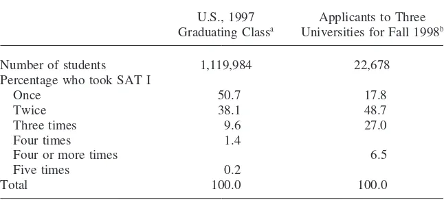
Table 1
Frequency of Retaking the SAT, All U.S. Test Takers and Applicants to Three Universities
U.S., 1997 Applicants to Three Graduating Classa Universities for Fall 1998b
Number of students 1,119,984 22,678
Percentage who took SAT I
Once 50.7 17.8
Twice 38.1 48.7
Three times 9.6 27.0
Four times 1.4
Four or more times 6.5
Five times 0.2
Total 100.0 100.0
a. Based on students who took SAT I one to five times in their junior or senior years. Source: College Board,Handbook for the SAT Program 1999–2000(1999), Table 6b.
b. Source: College Board and unpublished admissions data on 1998 applicants to three universities, au-thors’ calculations.
cite various kinds of bias and decry the test as an inappropriate apparatus for selecting a ruling class. ‘‘The Big Test,’’ as Lemann (1999) terms it, has drawn a significant amount of attention from academic researchers. Several studies have attempted to explain variation in SAT scores across states (Graham and Husted 1993) or individ-ual test takers (Dynarski 1985). SAT scores have frequently been used as an outcome measure in evaluating characteristics of school systems (Dynarski and Gleason 1993; Southwick and Gill 1997; Card and Payne 1998; see Hanushek and Taylor 1990, for a critique of this strategy) or a measure of ability (Ballou and Podgursky 1995). Additional research has investigated the predictive relationship between SAT scores and college outcomes (Boldt, Centra, and Courtney 1986; Bowen and Bok 1998; Rothstein 2002).
is not used universally, it is by far the most common among institutions that publicly reveal them.3
The second reason why retaking the SAT often pays off is the actual tendency for test takers to score higher when they retake the test. This tendency, revealed both in our data on applicants to three colleges and in nationwide College Board data, could theoretically be attributable to selection into the pool of retakers. We present evidence below to suggest that the gains associated with retaking the test are too large to be attributed to selection alone, and thus reflect benefits associated with familiarity or increases in knowledge between administrations.
From the standpoint of public policy, the subject of retaking is worth exploring for both equity and efficiency reasons. First, retaking is important to the extent that, in combination with the highest-score policy noted above, it affects admissions out-comes. It seems intuitive that the current highest-score policy provides an advantage to applicants with low costs of taking the test. Our results confirm this intuition. In light of the growing scrutiny of race-conscious college admissions criteria within the larger national debate over affirmative action, it is important to ask whether the ‘‘high-cost’’ applicants now disadvantaged by current policy are drawn selectively from certain groups—including racial minorities and the poor. If so, then the current policy almost surely warrants scrutiny.
Another reason to study retaking is allocative efficiency: such activity employs resources that have valuable alternative uses, and our results suggest that the current highest-score policy strongly encourages retaking.4 If colleges could obtain much the same information by following other policies that result in less test-taking, the current highest-score policy could justifiably be faulted as inefficient. It might be
3. We examined the admissions websites of the 50 top-ranked universities and the 50 top-ranked liberal arts colleges, according toU.S. News and World Report. Of fourteen that made a statement about how multiple SAT scores are treated in admissions decisions, ten explicitly stated the highest-score policy as described in the text, three specified the highest combined score at one sitting, and one said ‘‘primary consideration’’ would be given to the highest individual scores. Eight of the sampled colleges do not require the SAT, and the remainder stated no explicit policy on multiple scores.
The possibility exists, of course, that admissions committees, contrary to their stated policies, in practice make some adjustment in the case of applicants who have taken the test many times. Christopher Avery has shown us unpublished evidence that applicants who take more than one SAT are less likely to be admitted to selective colleges, controlling for their highest math and verbal scores and certain other characteristics. This evidence might indicate that multiple takers are penalized, or that multiple test tak-ing is correlated with negative factors observable to admissions officers but not econometricians. In any event, the magnitude of the penalty Avery observes is not sufficient to offset the benefits of retak-ing revealed below. The informal conversations we have had with admissions officers lead us to believe that most selective colleges do indeed follow the stated policy of using the highest math and verbal scores.
more efficient, for example, if colleges were to use the average of an applicant’s SAT scores instead of the highest, if such a policy reduced the amount of retaking without significant loss of information.5
This paper examines retaking and its consequences using data on the undergradu-ate applicants to three selective research universities. Section II describes the data and Section III examines the characteristics of those applicants who retake the SAT. We are especially interested in finding out whether the tendency to retake the SAT differs by gender, race, or socioeconomic status. The fourth section of the paper discusses the reasons why test scores tend to increase upon retaking. Section V dis-cusses a model of retaking. The applicant’s problem is analogous to one of optimal search: additional draws from a distribution of possible test scores can be had for a certain cost, and the applicant must decide whether the expected benefits of retaking exceed this cost. The sixth section reports the results of simulations that investigate the impact of college test score ranking policies on the frequency of retaking. The simulations are calibrated to match observed behavior under current policy. Alterna-tive test score ranking policies are compared along four criteria: accuracy (does rank-ing reflect true ability?), precision (are the rankrank-ing errors small?), bias (does the policy disproportionately favor certain groups?), and resource cost (how costly is the policy in terms of time and money spent taking the test?). Of nine policies com-pared, the current highest-score policy turns out to be the costliest, least accurate, and most biased. (It may serve other interests of colleges, however, as we note in the paper’s final section.) Following the simulations, we use our data to determine the impact that one particular policy change, limiting consideration to a student’s first SAT only, might have on applicant rankings. Section VII concludes the analysis. Although the data that we use are very instructive, two of their limitations should be noted at the outset. First, the institutions to which these data apply are not repre-sentative of all colleges and universities in the country. Thus, the results should be thought of as applying most to institutions with selective admissions. Second, no information is available in this data set on the potentially important activity of coach-ing and test preparation courses. If equity concerns are raised by differences between groups in the frequency of retaking, then differences in the access to test preparation courses should also be of concern.6 Given the nature of our data, we are simply unable to address this issue. Moreover, we would emphasize that our analysis is incomplete to the extent that it focuses on one aspect of behavior—retaking—but not on other aspects that might be involved as individuals respond to incentives created by colleges’ admissions policies. Two such aspects are decisions about when to take the test and what kinds of preparation to make before taking the test. We return to this issue in Section VII.
II. Data
The data used in the present analysis are based on first-year under-graduate applicants to three research universities in the South, two public and one private. All three are selective institutions. For the class enrolling in the fall of 1998, the three institutions accepted an average of 42 percent of their applicants, and their average yield rate was 50 percent.7All three require the SAT I as part of the complete application. For each applicant, information was obtained from the Educational Test-ing Service (ETS) from its Student Descriptive Questionnaire (SDQ), which is filled out by students taking the SAT. This questionnaire provides the applicant’s race, gender, residence, high school academic performance, and self-assessed ability as well as information on the income and education of the applicant’s parents. The ETS also provided a complete history of SAT scores, regardless of whether the student reported all those scores to the institution. These data were matched with information from the college applications.
The resulting sample included 22,678 students who applied to at least one of the three institutions for the fall of 1998 and who also took the SAT at least once.8Of these, more than 82 percent took the SAT at least twice, compared to the 49 percent who were multiple test-takers nationwide, as shown in Table 1. This large difference most likely reflects the comparatively selective character of the institutions in the current sample and therefore the possibly more competitive nature of the applicants to those institutions. The differences may be further influenced by the fact that rela-tively few applicants in the South take the ACT, as compared to the Midwest and West, where many applicants might conceivably be taking the SAT only once. What-ever the cause, this difference should be noted.
III. Who Retakes the SAT?
Table 2 presents distributions showing what kinds of students in our sample most often took the SAT multiple times. Retaking was significantly more common among students who receive lower scores on the first test administration. By gender, women were more likely to take the test more than once; whereas 20 percent of men took the test only once, only 16 percent of women did. Most of this difference is reflected in the percentages who took the test three times. By race, blacks were somewhat more likely to take the test multiple times (83.5 versus 82.2 percent). Hispanic applicants were about as likely as blacks to take the test more than once but less likely than blacks or whites to take it more than twice. The most distinctive racial group was Asian Americans, who exceeded all other groups in their rate of retaking. Whereas 32.5 percent of whites took the SAT three or more times, 42.6 percent of Asian Americans did. With respect to parents’ income, no very clear
7. Data fromPeterson’s Guide to 4 Year Colleges, 30th Edition(2000).
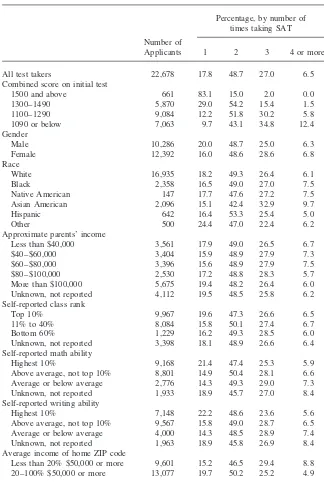
Table 2
Number of Times Taking SAT, by Selected Characteristics
Percentage, by number of times taking SAT
Number of
Applicants 1 2 3 4 or more
All test takers 22,678 17.8 48.7 27.0 6.5
Combined score on initial test
1500 and above 661 83.1 15.0 2.0 0.0
1300–1490 5,870 29.0 54.2 15.4 1.5
1100–1290 9,084 12.2 51.8 30.2 5.8
1090 or below 7,063 9.7 43.1 34.8 12.4
Gender
Male 10,286 20.0 48.7 25.0 6.3
Female 12,392 16.0 48.6 28.6 6.8
Race
White 16,935 18.2 49.3 26.4 6.1
Black 2,358 16.5 49.0 27.0 7.5
Native American 147 17.7 47.6 27.2 7.5
Asian American 2,096 15.1 42.4 32.9 9.7
Hispanic 642 16.4 53.3 25.4 5.0
Other 500 24.4 47.0 22.4 6.2
Approximate parents’ income
Less than $40,000 3,561 17.9 49.0 26.5 6.7
$40–$60,000 3,404 15.9 48.9 27.9 7.3
$60–$80,000 3,396 15.6 48.9 27.9 7.5
$80–$100,000 2,530 17.2 48.8 28.3 5.7
More than $100,000 5,675 19.4 48.2 26.4 6.0
Unknown, not reported 4,112 19.5 48.5 25.8 6.2 Self-reported class rank
Top 10% 9,967 19.6 47.3 26.6 6.5
11% to 40% 8,084 15.8 50.1 27.4 6.7
Bottom 60% 1,229 16.2 49.3 28.5 6.0
Unknown, not reported 3,398 18.1 48.9 26.6 6.4 Self-reported math ability
Highest 10% 9,168 21.4 47.4 25.3 5.9
Above average, not top 10% 8,801 14.9 50.4 28.1 6.6 Average or below average 2,776 14.3 49.3 29.0 7.3 Unknown, not reported 1,933 18.9 45.7 27.0 8.4 Self-reported writing ability
Highest 10% 7,148 22.2 48.6 23.6 5.6
Above average, not top 10% 9,567 15.8 49.0 28.7 6.5 Average or below average 4,000 14.3 48.5 28.9 7.4 Unknown, not reported 1,963 18.9 45.8 26.9 8.4 Average income of home ZIP code
Table 2(continued)
Percentage, by number of times taking SAT Number of
Applicants 1 2 3 4 or more
Urbanization of home ZIP code
Less than 80% urban 7,812 15.3 47.6 28.8 8.3
80–100% urban 14,866 19.2 49.2 26.0 5.6
Percentage black of home ZIP code
Less than 20% black 17,860 18.6 49.6 26.0 5.7
20–100% black 4,818 14.9 45.1 30.5 9.6
Note: Based on those who took the SAT at least once and graduated from high school in 1998. Row percentages may not add up to 100.0 due to rounding. Source: College Board and unpublished data on 1998 applicants to three universities, authors’ calculations.
patterns emerge.9Retaking was slightly more prevalent among applicants from fami-lies in the middle income categories, but the differences were not large. By contrast, the patterns of retaking differed markedly according to the student’s reported class rank. Those ranked in the top 10 percent of their high school class were least likely to take the test more than once. Applicants who ranked themselves among the highest 10 percent of students in either math or writing ability were significantly less likely to retake the test than those applicants with lower self-rankings.
The last three sets of categories shown in Table 2 apply to characteristics of the ZIP code where the student resided. Perhaps surprisingly, those in more affluent areas and in highly urbanized areas were less likely than others to take the test multiple times. With respect to the racial composition of ZIP codes, those living in areas with higher percentages of blacks were more likely to retake the SAT.
To summarize, Table 2 identifies several groups that were more likely than others to take the SAT multiple times: those with low initial scores, women, Asian Ameri-cans, those who rate themselves as average or below in ability, and those who live in less affluent, rural, or predominantly black neighborhoods. On their face, these simple correlations seem to dispel any notion that retaking is the exclusive or even preponderant domain of the affluent or urbanized.
For a fuller answer to the question of who retakes the test, it is necessary to examine the partial effects of various characteristics, holding other things constant. Our model, described in Section V below, suggests that there are three basic reasons why two individuals with the same initial test scores might be differentially likely to retake the test. First, individuals might have different expectations regarding the scores they would receive on the next test. Second, they may face different direct and indirect costs of retaking the test. Finally, they may attach different values to
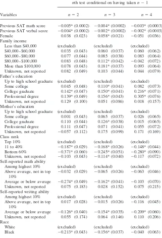
Table 3
Probit Equations Explaining Taking SAT at Least Two, Three or Four Times
Dependent variable: Indicator for whether applicant takes nth test conditional on having takenn⫺1
Variables n⫽2 n⫽3 n⫽4
Previous SAT math score ⫺0.005* (0.0002) ⫺0.004* (0.0002) ⫺0.003* (0.0003) Previous SAT verbal score ⫺0.004* (0.0002) ⫺0.002* (0.0002) ⫺0.002* (0.0003) Female 0.038 (0.023) 0.058* (0.021) ⫺0.051 (0.036) Family income
Less than $40,000 (excluded) (excluded) (excluded) $40,000–$60,000 0.035 (0.043) 0.060 (0.037) 0.060 (0.062) $60,000–$80,000 0.077 (0.044) 0.085 (0.038) 0.083 (0.064) $80,000–$100,000 0.083 (0.048) 0.112* (0.042) ⫺0.042 (0.072) More than $100,000 0.078 (0.043) 0.181* (0.037) 0.093 (0.064) Unknown, not reported 0.082 (0.049) 0.103 (0.044) 0.044 (0.079) Father’s education
Up to high school graduate (excluded) (excluded) (excluded) Some college 0.045 (0.048) 0.110* (0.041) 0.082 (0.073) College graduate 0.142* (0.047) 0.150* (0.041) 0.216* (0.071) Professional degree 0.139* (0.049) 0.156* (0.043) 0.305* (0.076) Unknown, not reported 0.129 (0.100) 0.051 (0.086) 0.018 (0.157) Mother’s education
Up to high school graduate (excluded) (excluded) (excluded) Some college 0.001 (0.043) 0.065 (0.037) 0.026 (0.065) College graduate 0.110 (0.044) 0.126* (0.038) 0.015 (0.065) Professional degree 0.111 (0.047) 0.071 (0.041) 0.055 (0.072) Unknown, not reported ⫺0.057 (0.112) 0.175 (0.099) 0.171 (0.169) Class rank
Top 10% (excluded) (excluded) (excluded)
11 to 40% ⫺0.187* (0.029) ⫺0.168* (0.026) ⫺0.148* (0.044) Bottom 60% ⫺0.371* (0.060) ⫺0.245* (0.051) ⫺0.280* (0.090) Unknown, not reported ⫺0.103 (0.043) ⫺0.114* (0.040) ⫺0.117 (0.072) Self-reported math ability
Among highest 10% (excluded) (excluded) (excluded) Above average, not in top ⫺0.032 (0.029) ⫺0.065 (0.026) ⫺0.063 (0.046)
10%
Average or below average ⫺0.274* (0.049) ⫺0.162* (0.041) ⫺0.103 (0.070) Unknown, not reported 0.075 (0.183) 0.028 (0.152) 0.075 (0.215) Self-reported writing ability
Among highest 10% (excluded) (excluded) (excluded) Above average, not in top 0.017 (0.028) ⫺0.015 (0.026) ⫺0.116 (0.045)
10%
Average or below average ⫺0.126* (0.040) ⫺0.154* (0.035) ⫺0.209* (0.060) Unknown, not reported 0.055 (0.174) 0.064 (0.146) 0.110 (0.206) Race
White (excluded) (excluded) (excluded)
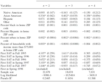
Table 3(continued)
Dependent variable: Indicator for whether applicant takes nth test conditional on having takenn⫺1
Variables n⫽2 n⫽3 n⫽4
Native American ⫺0.093 (0.147) ⫺0.163 (0.127) ⫺0.150 (0.212) Asian American 0.334* (0.042) 0.402* (0.035) 0.358* (0.056) Hispanic 0.071 (0.069) ⫺0.045 (0.063) 0.184 (0.115) Other 0.011 (0.070) 0.141 (0.072) 0.283 (0.125) Percent black in home ZIP 0.002 (0.001) 0.001 (0.001) 0.001 (0.001)
code
Percent Hispanic in home 0.002 (0.002) 0.003 (0.001) ⫺0.002 (0.002) ZIP code
Percent urban in home ZIP 0.002* (0.0004) 0.002* (0.0004) 0.002* (0.001) code
Percent of households with 0.003* (0.001) ⫺0.0001 (0.0008) ⫺0.004 (0.002) income more than $75,000
in home ZIP code
First SAT in Fall 1995 4.107* (0.259) 1.611* (0.418) 0.303 (0.652) First SAT in Spring 1996 4.319* (0.230) 1.418* (0.414) 0.209 (0.650) First SAT in Fall 1996 3.652* (0.213) 0.858 (0.412) ⫺0.375 (0.650) First SAT in Spring 1997 3.103* (0.209) 0.057 (0.412) ⫺0.857 (0.649) First SAT in Fall 1997 1.446* (0.210) ⫺0.935 (0.417) ⫺0.745 (0.672) First in Spring 1998 (excluded) (excluded) (excluded)
Sample size 22,678 18,638 7,631
Log likelihood ⫺8006.6 ⫺10,548.6 ⫺3418.0
Pseudo R2 0.2465 0.1636 0.1368
Notes: Table entries are probit coefficients. Standard errors are in parentheses. * denotes coefficients significant at the 1 percent level.
being admitted to a selective college. To examine the basic relationships between observed applicant characteristics and these underlying traits, Table 3 presents a series of probit equations explaining the decision to take the test twice, the decision to take the test a third time conditional on two administrations, and the decision to take it a fourth time conditional on three administrations. Included as explanatory variables are scores from the preceding test administration, gender, family income, father and mother’s education, self-reported class rank, self-reported math and writ-ing ability, race, and characteristics of the student’s ZIP code area. Finally, the equa-tions include dummy variables for the date of initial test administration.
the initial SAT test is associated with a decrease of 8 percentage points in the proba-bility of taking it a second time.10
Holding constant previous scores, family income now has a much clearer associa-tion than it appears to have in Table 2. Those whose parents made more than $60,000 had a 1.5 percentage point higher probability of retaking the test than those whose family incomes were below $40,000. Conditional on taking twice, applicants from these higher-income families were between 3.3 and 7 percentage points more likely to take the test a third time. Income does not significantly influence whether a three-time taker returns for a fourth test administration. Similarly, both mother’s and fa-ther’s education have a statistically significant effect, with those whose parents were college graduates more likely to retake the test, other things equal. As with income, the strongest effects of parental education appear in the decision to take the test a third time. Two-time takers whose fathers obtained a college degree were 6 percent-age points more likely to retake the test than otherwise identical applicants with a high-school-educated father. The marginal effect of mother’s education is of some-what smaller, though still significant, magnitude.
High school rank also has a significant association, with those in the top 10 percent being most likely to retake the test a second, third, or fourth time, with all other characteristics (including prior test scores) held constant. Similarly, those who as-signed relatively low ratings to their own math and writing ability were less likely to retake the test than those putting themselves in the top 10 percent. As with family income and parental education, the impact of class rank and self-assessment appears strongest in the decision to take the test a third time. In that case, either a class rank outside the top 10 percent, a low math self-assessment, or a low verbal self-assess-ment predicts a 6 to 9 percentage point decrease in the probability of retaking.
By race, blacks were less likely than whites to take the test two or three times. Other things equal, the probability of a black student taking the test at least twice was 4.5 percentage points less than that of an otherwise identical white student; conditional on taking the test twice, the black-white differential in the probability of taking the test a third time was 5.9 percentage points.11Asian Americans, on the other hand, were consistently more likely to retake the test: they were 5.5 percentage points more likely than an otherwise identical white student to take the test a second time. Conditional on taking twice, Asian applicants were 15.9 percentage points more likely to take the test a third time relative to otherwise identical white appli-cants. The test taking behavior of other racial or ethnic groups is not distinguishable from that of whites.
Applicants living in urban areas were more likely to retake the test a second, third or fourth time. As with many indicators, the strongest effect of urbanicity on retaking
10. Table 3 reports the actual probit coefficients, which have no natural interpretation. Our interpretation of the estimated effects in the test considers the impact of a unit change in one variable when all other variables are set equal to their means. In general, the effect of a variable on the probability of retaking will depend on the values of all variables in a probit equation.
occurs in the decision to take the test a third time, where an applicant from a com-pletely urban ZIP code was 8 percentage points more likely to retake the test than an applicant from a completely rural ZIP code. Other ZIP code characteristics, such as racial composition and income, do not display a consistent relationship with re-taking.
Finally, those who took their first SAT early were generally more likely than others to retake the test. This result is not surprising, since those applicants who initially took the SAT on a late date would simply not have had many chances to retake the exam.
In conclusion, the empirical analysis of who retakes the SAT indicates significant differences by race, income, parental education, self-reported class rank and ability, and type of community. Most of these relationships are obscured in the raw data, presumably by the extremely strong tendency for students who score well on the test to refrain from taking it again. These explanatory variables might measure differ-ential expectations regarding future test scores, variation in test-taking costs, or varia-tion in the benefits associated with admission. Many of the applicant characteristics associated with a lower propensity to retake are also correlated with lower overall SAT scores, suggesting that applicants may form expectations in a manner that re-sembles statistical discrimination.12The greatest amount of selection into the pool of retakers appears to occur in the decision to take the test a third time.
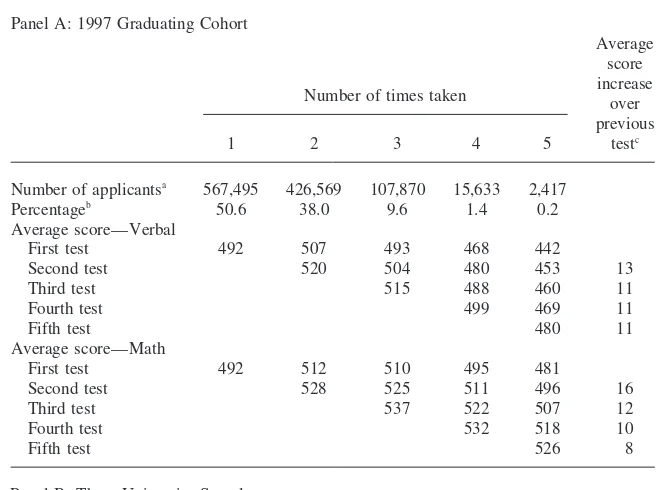
IV. Explaining the Increase in Scores
The tendency for SAT scores to increase is evident in the averages presented in Table 4. Using both nationwide data and data from our three-institution sample, the table shows that students taking the test on average improve their scores with each successive administration.13This tendency applies to both math and verbal tests. Consider, for example, those who took the SAT three times. Among all those in the 1997 national cohort, the average score among this group on the verbal test increased from 493 in the first taking to 515 on the third and from 510 to 537 on the math. Within our sample of applicants to three institutions, the comparable in-creases were 573 to 602 for the verbal and 555 to 583 for the math. For all those taking the test at least twice, the average increase on the second try in the national sample was 13 points for the verbal and 16 points for math. The comparable increases for the three-university sample were both about 16 points. Both samples show the same thing: retaking the test is associated with higher scores.
What explains these score increases? At least three possible reasons for this ten-dency suggest themselves. First, improvement might arise because of students’ creased familiarity with the SAT test, its format, and the kinds of questions it in-cludes. Second, rising scores may reflect the general increase in knowledge that one
12. A simple regression of first-time SAT scores on the covariates (other than SAT scores) in Table 3 reveals that income, parental education, class rank, self-reported math and writing ability, residence in an urban or wealthy ZIP code, and Asian racial background are all significantly positively correlated with test scores. Black, American Indian, Hispanic, and Female applicants receive significantly lower scores on their first test. The R2for this regression, with 22,678 observations, is 0.52.
Table 4
Average SAT Scores for Students, by Number of times Taking the test
Panel A: 1997 Graduating Cohort
Average score increase Number of times taken over
previous
1 2 3 4 5 testc
Number of applicantsa 567,495 426,569 107,870 15,633 2,417
Percentageb 50.6 38.0 9.6 1.4 0.2
Average score—Verbal
First test 492 507 493 468 442
Second test 520 504 480 453 13
Third test 515 488 460 11
Fourth test 499 469 11
Fifth test 480 11
Average score—Math
First test 492 512 510 495 481
Second test 528 525 511 496 16
Third test 537 522 507 12
Fourth test 532 518 10
Fifth test 526 8
Panel B: Three University Sample
Number of times taken Average score
increase over
1 2 3 4⫹ previous testc
Number of applicantsd 4,040 11,007 6,000 1,631
Percentageb 17.8 48.7 27.0 6.5
Average score—Verbal
First test 649 602 573 538
Second test 617 591 562 15.9
Third test 602 575 11.1
Fourth test 582 7.7
Average score—Math
First test 641 589 555 515
Second test 606 572 536 16.2
Third test 583 548 10.8
Fourth test 557 9.7
a. Data are based on 1,119,984 students who took the SAT1 one to five times in their junior or senior years.
b. Rows sum to 100.0.
c. Calculated for all those who took the test at least the indicated number of times.
expects to correspond to aging and time in school. Third, the increase could arise out of a selection effect, whereby those who had performed badly (relative to their expectations) constituted the bulk of retakers, in which case the improvement in their scores might arise from ordinary regression to the mean. The first two possible causes could be thought of as ‘‘real,’’ as opposed to mere selection.
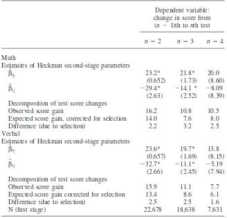
Determining whether scores truly tend to ‘‘drift upward’’ upon retaking is an important precursor to modeling retaking behavior. To test whether the observed increases in test scores are consistent with selection effects, we employ the two-stage Heckman sample-selection procedure (Heckman 1979).14The first stage of the procedure consists of probit regressions identical to those reported in Table 3 above, which predict the probability that any particular applicant will enter the sample of retakers. In the second stage, we estimate the following equations for both math and verbal test scores:
(1) (Predicted Test Score Gain)ij ⫽βˆ0j⫹βˆ1jλˆi,
whereiindexes students,jrepresents either the verbal or math score, andλˆiis an applicant’s inverse Mills ratio as estimated by the first-stage probit regression.15This procedure allows us to predict selection-corrected test score gains for applicants both in and out of sample.16Table 5 presents estimates ofβˆ
0jandβˆ1j.
We estimate separate second-stage equations for test score changes from the first to the second, second to third, and third to fourth test administrations; one set each is estimated for the verbal and math parts of the test. For all six equations, the selection coefficientβˆ1jis negative, indicating that, as theory would predict, those individuals most likely to retake the test are those with the highest expected score gains. Esti-mates of selection into the pool of two- and three-time takers are statistically signifi-cant; selection into the pool of four-time takers is not.
To give an idea of the importance of this selection effect on the amount of gains, we use the second-stage Heckman results to calculate simple predicted score changes between thenth and (n⫹1)th administrations for all individuals who took thenth test, regardless of whether they actually took the (n⫹1)th. We compare these selection-corrected average test score gains with the observed average score gain, equating the difference in these values with a selection effect.
14. The Heckman selection correction procedure presumes that the error terms in the sample selection equation (the probit equations reported in Table 3) and the outcome equations (where outcomes here are increases in test scores) follow a bivariate normal distribution, with some correlation between the error terms. In other words, individuals with exceptionally low (latent) increases in test scores might also be exceptionally unlikely to retake the test.
15. The inverse Mills ratio for each observation is computed as follows:
λˆi⫽
φ(xiγˆ)
Φ(xiγˆ)
wherexiis the vector of characteristics included on the right hand side of the probit equation,γˆ is the vector of estimated coefficients, andφandΦare the density and cumulative density of the standard normal distribution, respectively. Relatively low values of the inverse Mills ratio in this case correspond to individ-uals with a relatively high probability of retaking the test.
Table 5
Explaining Improvement in SAT Scores and the Role of Selection for Those Taking SAT at Least Two, Three, or Four Times
Dependent variable: change in score from
(n⫺1)th tonth test
n⫽2 n⫽3 n⫽4
Math
Estimates of Heckman second-stage parameters
βˆ0j 23.2* 21.8* 20.0
(0.652) (1.73) (8.60)
βˆ1j ⫺29.4* ⫺14.1 * ⫺8.09
(2.63) (2.52) (8.39)
Decomposition of test score changes
Observed score gain 16.2 10.8 10.5
Expected score gain, corrected for selection 14.0 7.6 8.0
Difference (due to selection) 2.2 3.2 2.5
Verbal
Estimates of Heckman second-stage parameters
βˆ0j 23.6* 19.7* 13.8
(0.657) (1.69) (8.15)
βˆ1j ⫺32.7* ⫺11.1* ⫺5.19
(2.66) (2.45) (7.94)
Decomposition of test score changes
Observed score gain 15.9 11.1 7.7
Expected score gain corrected for selection 13.4 8.6 6.1
Difference (due to selection) 2.5 2.5 1.6
N (first stage) 22,678 18,638 7,631
Note: Standard errors in parentheses.
* denotes coefficients significant at the 1 percent level.
Consistent with the negative point estimates ofβˆ1j, at least part of observed test score gains can be attributed to selection into the pool of applicants in all six cases. This procedure also shows, however, that most of the observed gain in test scores associated with retaking cannot be attributed to selection. Between 70 and 90 percent of the observed test score gain in each instance is robust to selection correction.17
These residual test score gains can be considered real and attributable either to a gain from familiarity with the test or to gains due to learning more over time.18
V. Model and Implications
To better understand the origins and implications of retaking and to consider how behavior might change under alternative policy regimes, it is helpful to think about what goes into the decision to retake the test. We find it useful to begin by thinking of the SAT as simply a series of questions designed so that a given student faces the same probabilityρof answering each question correctly. We refer toρas true ‘‘ability,’’ although by using this term we do not mean to weigh in on the question of what exactly the test does measure. In this case, the percentage of questions a student actually answers correctly,p, is an estimate of the true parame-ter ρ. As described, this setup is equivalent to a series of Bernoulli trials, and the distribution ofpis given by a binomial. We extend this logic to two different kinds of ability, mathematical and verbal, with the student’s true mathematical abilityρm and true verbal abilityρv. Following the binomial analogy, we assume the population distribution of these parameters falls between zero and one, with the potential that these two ability measures may be correlated with one another. Importantly, we also assume that applicants do not know their true ability parameters, but make inferences about them on the basis of information received through test scores and other sources. We envision a simple admissions process in which the college’s admissions office attempts to rank its applicants according to ability, based on the point estimates received through applicant test scores. The applicant’s objective in deciding how many times to take the test is to maximize the probability of admission, subject to cost-related constraints. Consistent with the notion that applicant ability as measured by the SAT is not the only criterion for admission, we presume that there is no set of SAT scores that guarantees admission.
Applicants who retake the SAT are effectively submitting multiple point estimates of their true mathematical and verbal ability. It is clear that applicants’ incentives to retake the test will be influenced by how a college treats these multiple point estimates. Were colleges to accept only the first set of point estimates, {p1
m,p1v}, then applicants would never retake the test, so long as the cost of taking the test were positive. When colleges consider point estimates other than the first set in determining their ranking, students can be expected to retake the test whenever they believe the benefits of doing so will exceed the costs.
The highest-score policy commonly used by college admissions offices translates into the following rule: for a student who has taken the testntimes, use the maximum
mathematical score, max {p1
m, . . . , pnm}and the maximum verbal score, max{p1v, . . . ,pnv}as point estimates ofρmandρv. Applicants will choose to retake the test when they judge that the increase in the probability of admission associated with expected changes in either their mathematical or verbal score is sufficiently large to justify the costs of retaking. The applicant’s problem becomes analogous to one of optimal search with the possibility of recall (Stigler 1961, DeGroot 1968). An appli-cant who faces dollar-denominated test-taking costs, including fees, opportunity costs, and psychic costs, equal toc, places a dollar valueVon admission, and has received maximum math and verbal scores ofp*mandp*v in their previous test admin-istrations will retake the test if and only if:
(2)
冱
f(pm) is the applicant-specific probability density function for math point estimates, andf(pv) is the corresponding probability density for verbal point estimates.19 Imbed-ded in the equation is the assumption that in each test administration, the point esti-matespmandpvare drawn independently from their respective marginal distributions. The equation also assumes that the point estimates take on a finite number of val-ues—a reasonable assumption, since there are only 61 unique scores on the SAT math and verbal scales.20
If applicants knew the value of their underlying ability parameters with certainty, their optimal decision would be to continue taking the test until they had achieved some ‘‘reservation test score.’’21But because we presume that students donotknow their underlying ability parameter with certainty, the typical reservation test score rule will not apply (Rothschild 1974).To determine an applicant’s decision rule in this scenario, we presume that applicants receive and process information in a Bayes-ian manner.
We begin by assuming that applicants receive prior information regarding their subjective distributions off(ρm) andf(ρv) by receiving ‘‘practice draws’’—pre–test administration Bernoulli trials that might be thought of as information contained in school grades, previous standardized test scores, and the like. Along with the scores from their first test administration, these draws form their information set as they decide whether to take the test a second time. Based on the information contained in their first test scores and practice draws, applicants form a posterior probability distribution for the underlying parameters for use in their decision on whether to retake the test. Following any subsequent test administrations, applicants once again
19. We assume here that all applicants face the same acceptance probabilities,a(pm,pv). The simulation
we perform is unaffected if the acceptance probability surface mapped in Figure A2 shifts up or down uniformly. To the extent, however, that the acceptance probability surface differs substantially in shape across categories of applicants, we are overlooking an important source of variation in behavior. Affirma-tive action programs, for example, may result in a leveling up in the admission probability surface for some groups, which might in turn explain their reduced likelihood of retaking the test.
20. Scores range from 200 to 800 in increments of 10.
21. Because there are two elements to the SAT score, there would be no unconditional reservation values ofpmorpv. Rather there would be conditional reservation values: the value ofpmthat will induce an
update their posterior probability distributions. As changes in an applicant’s beliefs about her true ability influence the probability she attaches to receiving any particular test score, her ‘‘reservation test scores’’ may change over time.
Two applicants who receive identical scores on their first test may be differentially likely to retake the test for three basic reasons. First, they may face different costs of retaking the test. Those with part-time jobs, for instance, will tend to face higher opportunity costs of taking a test than other applicants. Applicants may have differen-tial psychic costs of undergoing a testing procedure. Even testing fees themselves, which are generally constant, may impose differential utility costs. Second, the value they attach to being admitted to a college may differ. These first two factors can be consolidated into one: applicants may differ in the ratio of their test-taking costs to the benefits they attach to admission—the ratioc/V. Third, their prior beliefs, based on their practice draws, may lead them to expect different scores on their next test.
VI. Simulating Test-Taking Behavior
There are two basic reasons to simulate test-taking behavior. First, simulations provide further evidence on the relationship between an applicant’s re-taking behavior, the test-re-taking costs faced, the benefits attached to being admitted, and prior beliefs under the current policy. Second, simulations allow us to predict the impact of changes in SAT score ranking policy without actually ‘‘living through’’ the alternative policies.
A. Calibration and Results under the Current Policy
The simulation exercise we undertake here is calibrated in the sense that we choose parameter values that result in simulated behavior under the current SAT score rank-ing policy that closely resembles actually observed behavior under that same policy. To the extent that our simulation provides a reasonable facsimile of reality as ob-served in actual data, we have confidence that the procedure can suggest what changes in behavior might reasonably be associated with policy changes.
The simulation procedure involves the following steps:
1. For each of 1,000 simulated applicants, draw a value for ρm andρv, the applicant’s true math and verbal ability. We derive the population distribu-tion of values forρmandρvfrom our data on applicants to three selective universities. Specifically, these values are based on the distribution of first-time SAT scores in our data.22Scores are translated into ability parameters first by subtracting 200 (the minimum score) from each, then dividing the
result by 600.23By deriving ability parameters directly from applicant SAT scores in our data, we are assuming thatρmandρveach take on one of 61 discrete values, like the scores themselves.
2. Randomly draw an initial value of c/V, the ratio of costs of test-taking to benefits of admission, for each applicant. For simplicity, the cost-to-benefit ratio will take on two values corresponding to ‘‘high cost’’ and ‘‘low cost’’ applicants. The values of c/V are calibrated to yield a pattern of retaking similar to that found in our data. In this simulation, the ratio of test taking costs to admission benefits increases linearly in the number of times previ-ously taken.
3. Administer 120 ‘‘practice’’ Bernoulli trials, 60 each with probability of suc-cessρmandρv. Using the results of these practice trials, each applicant forms a prior probability distribution that indicates their perception of their own ability prior to any actual test-taking. Applicants will never learn their true ability parameters; they will only receive information about them based on how they perform on tests.
4. Administer a simulated SAT, which consists of 60 independent Bernoulli trials each for the math and verbal scores, with probability of success equal toρmandρv, respectively.24Calculate the applicants’ SAT scores by multi-plying the number of successes by 10, then adding 200. Applicants then update their beliefs regarding the true values of their ability parametersρm andρv.
5. Applicants use their newly calculated posterior distribution on ρm andρv, their value ofc/V, and probabilities of admission conditional on test scores to decide whether to retake the SAT. Applicants are aware that they can expect their scores to drift upwards if they decide to retake. If applicants decide to refrain from retaking the test, the simulation stops.
6. For applicants that decide to retake the SAT, we administer an additional simulated SAT. Because our evidence presented in Section IV above indi-cates that individuals’ scores increase upon retaking, we increase the proba-bilities of success on the math and verbal exams. These increases inρmand ρvreflect the presumption that each time an applicant retakes the SAT, she can expect both her math and verbal scores to increase by about 10 points. Applicants use the information in their newest set of SAT scores to update their beliefs regardingρmandρv, then return to Step 5.
23. There are two exceptions to this translation. SAT scores of 800 are translated into ability parameters of 0.99 rather than l, and SAT scores of 200 are translated into ability parameters of 0.01 rather than 0. Setting ability parameters equal to zero or one in our simulation exercise would eliminate all uncertainty in an applicant’s test scores.
Table 6
Simulation Results under the Current Score Ranking Policy
One-time Two-time Three-time Four-time takers takers takers takers
First scores math/verbal 585/600 565/581 601/611 588/613 Second scores math/verbal 580/601 610/617 593/620
Third scores math/verbal 626/637 595/623
Fourth scores math/verbal 623/644
Percent of sample 13.5% 48.2% 28.7% 9.6%
Mean true ability parameters math/verbal 573/582 570/587 604/614 586/610 Percent ‘‘high-cost’’ type 35% 19% 8% 0%
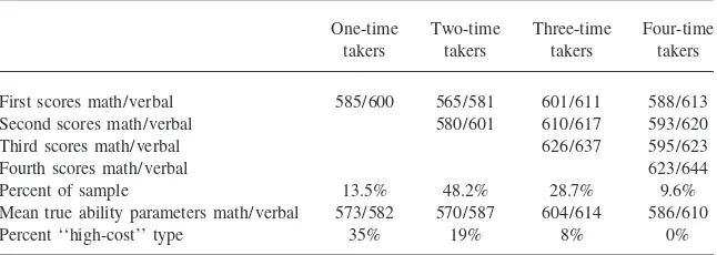
Details regarding the specific assumptions and parameter values used in the simu-lation can be found in the Appendix. The simusimu-lation was calibrated to match the probability of a simulated applicant taking the test a second, third, or fourth time to the observed probability of an applicant’s taking the test a second, third, or fourth time. As Table 6 shows, the calibration exercise performed relatively well in match-ing the observed probability of retakmatch-ing. Among our simulated applicants, the proba-bility of taking the SAT two or more times under the current score ranking policy is 86.5 percent; the probability of taking the SAT three or more times is 38.3 percent, and the probability of taking the SAT four times is 9.6 percent. Since very few actual applicants take the SAT five or more times, our simulation stops after the fourth test administration.
A comparison of Tables 4 and 6 suggests that our simulation fails to capture the exact nature of selection into the pool of retakers in two ways. First, in our data on actual applicants, the set of individuals stopping after one test administration obtains significantly higher scores, on average, than any other group. In our simulation, that is not the case. Second, our simulation suggests that applicants with exceptionally high test score gains are more likely to refrain from taking the test an additional time. Individuals who experience moderate increases, conversely, are more likely to take the test again. In our actual data, test score gains are spread more evenly through the population: the set of individuals who stop after the third administration, for example, experience roughly the same gain between the 2nd and 3rd administra-tions as do those who choose to take the test a fourth time.
overesti-mate the extent of the retaking in the general population—implying that our simu-lated applicants must score higher, relative to expectations, than actual applicants before deciding to stop taking the test.
This caveat should be considered carefully for two reasons. First, it implies that our simulation may not perfectly capture the degree of applicant response to changes in SAT score ranking policies. Second, it suggests that we are omitting one important source of applicant response to a change in test score ranking policies: the decision to apply in the first place. Bearing these concerns in mind, we will proceed with our analysis of simulation results.
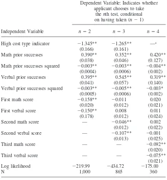
Table 7 examines the determinants of retaking by presenting probit regressions analogous to the ones performed with actual data in Table 3 above. The first result, which predicts the probability of an applicant deciding to take the test a second time, indicates that cost-to-benefit ratios, prior beliefs, and first test scores each enter significantly into the equation. Comparing a high-cost and low-cost applicant with all other variables alike and equal to the mean values, the high-cost applicant is 20 percent less likely to retake the test. When all other variables are set equal to their respective means, an increase of 50 points in both the SAT math score and verbal score reduces the probability of retaking by about ten percentage points—a magni-tude quite similar to that derived from our actual data. Prior beliefs display a qua-dratic relationship with retaking behavior. For most applicants, the probability of retaking increases as the number of practice trial successes increases. This tendency decreases as the number of practice successes approaches the maximum value of 60. Holding other things constant then, applicants with more ‘‘pessimistic’’ prior beliefs are less likely to retake the test.
These basic results persist when analyzing the decision to take the test a third time or a fourth time. With each retaking, a greater fraction of high-cost types drop out. A high-cost applicant with mean values of all other variables is about 36 percent less likely to take the test a third time when compared to an identical low-cost appli-cant. As shown in Table 6, no high cost applicants choose to take the test a fourth time. These results bear a distinct resemblance to those discussed in Section III above, which indicated that the greatest degree of selection occurred in the decision to take the test a third time conditional on taking twice.
Interestingly, the probability of retaking the test appears to depend only on the most recently obtained set of SAT scores. Controlling for the most recent scores, previously received scores do not significantly affect the probability of retaking. Prior beliefs continue to significantly affect retaking, however.
Table 7
Explaining Retaking Behavior in Simulated Data
Dependent Variable: Indicates whether applicant chooses to take
thenth test, conditional on having taken (n⫺1)
Independent Variable n⫽2 n⫽3 n⫽4
High cost type indicator ⫺1.345** ⫺1.265** —a
(0.166) (0.161)
Math prior successes 0.390** 0.352** 0.420**
(0.038) (0.046) (0.127)
Math prior successes squared ⫺0.003** ⫺0.003** ⫺0.004**
(0.0004) (0.0006) (0.002)
Verbal prior successes 0.395** 0.545** 0.319**
(0.041) (0.057) (0.140)
Verbal prior successes squared ⫺0.003** ⫺0.005** ⫺0.003*
(0.0005) (0.0006) (0.002)
First math score ⫺0.158** ⫺0.011 0.020
(0.020) (0.012) (0.021)
First verbal score ⫺0.150** 0.008 0.011
(0.178) (0.012) (0.024)
Second math score — ⫺0.046** 0.002
(0.012) (0.022)
Second verbal score — ⫺0.107** ⫺0.001
(0.013) (0.025)
Third math score — — ⫺0.092**
(0.020)
Third verbal score — — ⫺0.075**
(0.021)
Log likelihood ⫺219.99 ⫺434.72 ⫺175.00
N 1,000 865 360
Note: Standard errors in parentheses. Coefficients are derived from probit estimation of each equation. Test scores and number of prior successes each take on integer values between 0 and 60.
** Denotes a coefficient significant at the 5 percent level, * the 10 percent level.
B. Evaluating the Current Score Ranking Policy
Our data on simulated applicants has one central advantage over data on actual appli-cants: we are able to observe the ability parameter that SAT scores are intended to estimate. We can therefore examine the effectiveness of current and alternative col-lege test score ranking policies in providing a high-quality point estimate of an appli-cant’s true ability. We use four different criteria to determine the quality of a ranking policy.
1. Accuracy. This is simply the average difference between the estimate of an ability parameter derived from a policy and the true value of that parameter (‘‘ranking error’’). Both positive and negative values are theoretically pos-sible.
2. Precision. This measure equals the standard deviation of ranking errors asso-ciated with a particular policy. A policy can be inaccurate yet precise, if ranking errors are more or less the same for all applicants. An imprecise policy is one where the ranking errors vary quite a bit from applicant to applicant. Precision can never be negative; values closer to zero are prefera-ble, other things equal.
3. Bias. This measure should not be confused with accuracy, which in a statisti-cal sense could be referred to as biasedness. Here, we refer to bias as the degree to which the test score ranking policy places high–test taking cost types at a disadvantage. It equals the difference between the average ranking error for low-cost types and the average ranking error for high-cost types. We presume that zero is the most preferred bias value.25
4. Cost. The cost of a ranking policy is simply the average number of test administrations per applicant observed under that policy. Other things equal, a ranking policy that induces a lower frequency of test-taking is considered superior. In using this criterion, we presume that the value of resources con-sumed in retaking the test exceeds the value of any benefits, such as learning, that accrue to the applicant in the process.
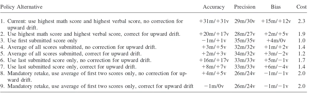
Table 8 presents our calculations of the accuracy, precision, bias and cost of the most common current SAT score ranking policy, along with those of several alterna-tive policies to be discussed in the following section.
Under the current SAT score ranking policy, our simulation suggests that admis-sions officers’ point estimate of the typical applicant’s ability is significantly higher than the true value.26The average deviation between the test score used to estimate an applicant’s ability and that applicant’s true ability, which we define as the
‘‘rank-25. It is conceivable that colleges might wish to implement a biased score ranking policy. Recall that it is not possible to separate individuals with a high test taking cost from those who place a low value on admission. If colleges determined that variation in benefits were much more important than variation in costs, and they wished to provide an advantage to students attaching the highest value to admission, then a biased policy would appear attractive.
Vigdor
and
Clotfelter
23
Comparing Student Test Score Ranking Policies
Policy Alternative Accuracy Precision Bias Cost
1. Current: use highest math score and highest verbal score, no correction for ⫹31m/⫹31v 29m/30v ⫹15m/⫹12v 2.3
upward drift.
2. Use highest math score and highest verbal score, correct for upward drift. ⫹20m/⫹17v 28m/27v ⫹2m/⫹5v 1.9
3. Use first submitted score only ⫺1m/⫹1v 35m/35v ⫹4m/0v 1.0
4. Average of all scores submitted, no correction for upward drift. ⫹3m/⫹5v 32m/32v ⫹1m/⫹2v 1.4
5. Average of all scores submitted, correct for upward drift. ⫹2m/⫹3v 34m/32v ⫹3m/⫺2v 1.2
6. Use last submitted score only, no correction for upward drift. ⫹16m/⫹17v 33m/33v ⫹5m/⫺1v 1.7
7. Use last submitted score only, correct for upward drift. ⫹8m/⫹7v 33m/33v ⫹6m/⫺4v 1.4
8. Mandatory retake, use average of first two scores only, no correction for up- ⫹4m/⫹5v 26m/24v ⫺1m/⫺1v 2.0
ward drift.
9. Mandatory retake, use average of first two scores only, correct for upward drift ⫺1m/0v 26m/24v ⫺1m/⫺1v 2.0
ing error,’’ is approximately 30 points on the verbal scale and 30 points on the math scale. Because current policy effectively picks the most positive outlier among competing point estimates, it is not surprising that applicants are consistently rated above their true ability. The tendency for scores to drift upward upon retaking exacer-bates ranking errors.
Ranking errors also differ appreciably among applicants under the current policy. The precision values convey this basic fact, and the bias values show one component of the variance in ranking errors across applicants. In our simulation, high-cost appli-cants, who were approximately 20 percent less likely to retake the test and 36 percent less likely to take the test a third time conditional on taking twice, are consistently ranked lower than low-cost applicants of equal true ability. By taking the test more frequently, low-cost applicants are receiving more chances to draw a positive outlier from their distribution of possible test scores. These applicants also are more likely to benefit from upward drift in test scores. If applicants are ranked according to the sum of their math and verbal scores, the average high-cost applicant in this simula-tion is placed at a 27-point disadvantage relative to an equivalent low-cost rival.
Finally, the current policy leads to a situation where the average applicant takes the test 2.3 times. By construction, this value is observed both in our simulated data and in our actual data on applicants to selective colleges.
C. Evaluating Alternative Score Ranking Policies
Table 8 goes on to present the results of additional simulations under different test score ranking policies. For each policy, it is necessary to repeat the simulation since changes in ranking policies, by altering the potential benefits from retaking the test, will influence applicant behavior. There are a total of eight proposed alternative policies to consider.
Policy 2: Correct for upward drift in test scores
One alternative to current policy would be to deflate second and subsequent test scores to reflect the fact that scores tend to increase upon retaking. Before choosing an applicant’s highest math score and highest verbal score, second and subsequent test scores are corrected, so that they are drawn from the same distribution as the first submitted score.
Because this policy reduces the potential benefits of retaking the test, it is not surprising that the average number of test administrations per simulated applicant decreases. The typical applicant now takes the test 1.9 times, rather than 2.3. The policy also achieves a noteworthy reduction in bias—high-cost types are now at a seven-point rather than 27-point disadvantage. Accuracy improves somewhat, though estimates of the average applicant’s ability still exceed the true value by roughly 40 points. Precision improves slightly. Overall, this policy alternative ranks higher than the current policy on all dimensions.
Policy 3: Use only the first submitted score
would equal zero if the simulation’s sample size were large enough. The principal disadvantage of this policy is a reduction in precision, since most applicants are taking the test fewer times, there is simply less information to use in the creation of a point estimate. Relative to previously considered policies, the standard deviation of ranking errors under this alternative is roughly 25 percent higher. The cost savings, accuracy improvement, and elimination of bias achieved under this policy must therefore be weighed against the loss in precision.
Policies 4 and 5: Use the average of all scores submitted.
Under this policy, an applicant’s decision to retake the test is based on a different calculation than that presented in Equation 2 above. Using the same notation as in Section III, the applicant deciding to take the test for the nth time must determine whether
wherep¯mandp¯vare the average of all previous math and verbal scores, respectively. This is a fundamentally different situation than in the previous case. Under current policy, it is not possible for an applicant’s ranking to decrease after retaking the test. Under this alternative, the applicant’s ranking may decrease if either the math or verbal score on the final test is lower than the average of scores on all previous tests. The simulation procedure, altered to reflect the new calculation in Equation 2, suggests that applicants would respond to this increase in downside risk by dramati-cally reducing the frequency with which they retake the test. When scores are not corrected for upward drift, the average applicant takes the test 1.4 times. Bias and accuracy are also greatly improved under this policy, even without correction for upward drift. Policy 5, which combines this revision of policy with the correction for upward drift described above, reduces test administrations to 1.2 per applicant, virtually eliminates bias, and attains near-perfect accuracy. Both policies feature the same drawback: a decrease in precision associated with collecting less information on each applicant. As with Policy 3, it is necessary to weigh the accuracy, bias and cost gains against the losses in precision when ranking these alternatives against current policy.
The reduction in retaking under the average score policy can be empirically cor-roborated by comparing the behavior of SAT takers with that of Law School Admis-sion Test (LSAT) takers. The most common test score ranking policy among law schools is to use the average of all submitted scores.27As these simulation results would suggest, the rate of retaking among law school applicants is significantly less than that among college applicants nationwide. Fewer than 20 percent of law school applicants take the LSAT more than once.28
Policies 6 and 7: Use only the last submitted score.
These policies change applicants’ incentives once again. Rather than perform the
27. In a survey of admissions websites for the top 20 law schools as ranked inUS News and World Report, nine schools explicitly stated policies for treating multiple scores. Of these, eight used the average score policy. The ninth school used the highest-score policy. The Law School Admissions Council advises mem-ber schools to use the average score policy.
cost-benefit comparison in Equation 2, applicants deciding whether to take the test annth time will now determine whether
(4)
冱
pm
冱
pv
V
冢
a(pnm,pnv)⫺a(pnm⫺1,pvn⫺1)
冣
f(pm)f(pv)⬎c,where superscripts indicate the test administration from which scores are derived. As in the preceding case, applicants now face the possibility of a decrease in ranking upon retaking. Following the analogy to a search model, this policy would eliminate the possibility of recall.
It is interesting to compare the versions of this policy that omit or include the upward-drift correction to Policies 4 and 5 above. Although the last-score policies outperform current policy in terms of cost, accuracy and bias, they are strictly inferior to the test-score averaging policies on all measures. They share similar precision values with the score-averaging policies.
Policies 8 and 9: Use exactly two scores for each applicant.
The final alternative policy involves a ‘‘mandatory retake’’ for all applicants. Like the first-score-only policy, this one eliminates the role of the applicant in determining test-taking strategy. As with that earlier policy, this one eliminates the potential for bias; perfect accuracy is attained in the version of the policy that corrects the second score for upward drift. This policy, with or without upward drift correction, achieves the best precision ranking of any alternatives. Mandating additional retakings would further improve the precision of the final ranking.
Because no single policy offers the best combination of accuracy, precision, bias, and cost, ranking the score-ranking policies is inherently a subjective matter. The one clear comparison that can be made here involves the current policy, which is strictly dominated along all four measures by both Policy 8 and Policy 9—the man-datory-retake policies that average exactly two test scores from each applicant, with or without correction for upward drift in the second score. These alternatives are less costly, less biased, more accurate, and more precise than current policy.29Other alternatives may in turn be preferred to these, depending on the degree to which policymakers are willing to exchange greater precision for lower costs.
D. Importance of Existing Bias
The simulation-based comparisons offered in the preceding section imply that certain SAT takers—those with high test-taking costs—are placed at a disadvantage by the common practice of colleges to use the highest submitted scores as point estimates of ability. Because test-taking costs are not directly observed, the question of how policy changes would affect particular observable groups, such as the socioeconomi-cally disadvantaged or racial minorities, remains open. Disadvantaged groups may
retake the test less frequently, conditional on initial scores, because their costs of retaking are higher, or because their expectations of performance on later tests are more pessimistic. In the former case, policy changes might improve the standing of groups with low conditional retake probabilities. In the latter case, so long as expecta-tions are not systematically biased within groups, policy changes would have little effect.
To provide some insight as to the implications of test score ranking policies for certain observable groups, we can perform one hypothetical experiment with our data on applicants to three universities. As discussed in the previous section, it is inappropriate to gauge the impact of test score ranking policies using actual data, because the data generation process is itself a function of the policy in place. The one alternative policy that would seem to be nearly exempt from this concern is Policy 3, which considers an applicant’s first score only. Applicants could only re-spond to this policy by altering the date of their test administration. By examining the set of applicants who first took the test within a narrow range of dates, we can infer the impact of switching to a policy that would have constrained those applicants to submit no other scores after the first.30In essence, we are considering the impact of changing the SAT to resemble the PSAT, a test administered to all takers on a uniform date nationwide. The range of dates we consider includes January, March, and May of 1997.
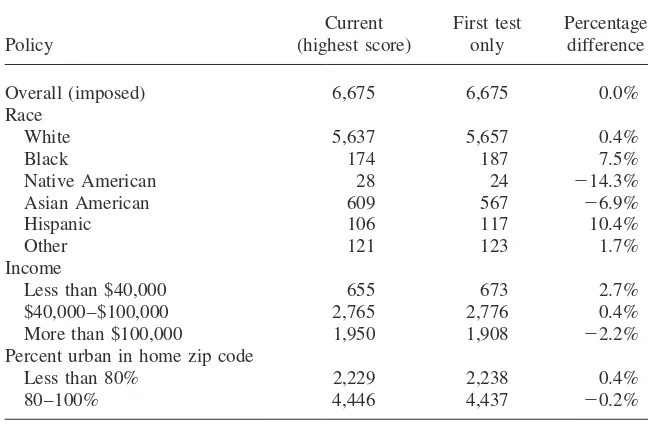
To gauge the potential impact of SAT ranking policy on actual admission deci-sions, we constructed a simple simulated acceptance rule. Using overall acceptance rates for each institution, we calculated a putative number of acceptances for each test administration date and institution. Sorting applicants by their combined math and verbal scores, those who ranked high enough to be in that number for each test date and institution were deemed ‘‘accepted.’’ We then pooled all three groups of putatively accepted students for each of the three dates and divided them according to race, family income, and percent urban in their home ZIP code. (Note that an individual applying to more than one institution could be deemed an acceptance to more than one institution.) We ranked the applicants to each institution first ac-cording to the highest-score rule and second acac-cording to the first-score-only rule. The resulting average characteristics of the pool of ‘‘accepted’’ applicants are shown in Table 9. Unsurprisingly, a shift from the current policy to a first-test-score-only rule increases the probability of admission among those groups less likely to retake the test controlling for initial scores (African-Americans, Hispanics, families with lower incomes) and decreases the probability among groups more likely to retake the test controlling for initial scores (higher income families, Asian-Ameri-cans). The magnitude of these changes in acceptance rate is noticeable, if not over-whelming. Acceptance rates for black applicants increase almost 8 percent under the first-score ranking relative to the highest-score ranking. The impact on acceptance for lower-income applicants is somewhat smaller. The table makes an important point: even if a ranking policy places certain groups at a relative disadvantage, the
Table 9
Effect of Current (Highest-Score) Policy on Acceptance Rates: Simulations for Three Universities (weighted average of acceptance rates, by category)
Current First test Percentage
Policy (highest score) only difference
Overall (imposed) 6,675 6,675 0.0%
Race
White 5,637 5,657 0.4%
Black 174 187 7.5%
Native American 28 24 ⫺14.3%
Asian American 609 567 ⫺6.9%
Hispanic 106 117 10.4%
Other 121 123 1.7%
Income
Less than $40,000 655 673 2.7%
$40,000–$100,000 2,765 2,776 0.4%
More than $100,000 1,950 1,908 ⫺2.2%
Percent urban in home zip code
Less than 80% 2,229 2,238 0.4%
80–100% 4,446 4,437 ⫺0.2%
number of individuals truly affected by the policy—those who are on the border between acceptance and rejection—makes up only a small component of the overall applicant pool. Nonetheless, it is important to consider the impact of the highest-score policy. In an era of decline in affirmative action policies, any policy which places African-American applicants at a disadvantage, even if only an 8 percent disadvantage, merits scrutiny. It is also conceivable that applicants occupying other segments of the test score distribution might be disadvantaged in decisions other than admission, especially financial aid rankings.
It is also worth emphasizing that this exercise was undertaken using data on appli-cants to three selective colleges. To the extent that changes in test score ranking policies lead to changes in individual decisions to apply to selective colleges, this exercise will understate the true effect of changing policies.