Manajemen | Fakultas Ekonomi Universitas Maritim Raja Ali Haji 322.full

(1)

Wealth

Dynamics

in the 1980s and

1990s

Sweden and the United States

N. Anders Klevmarken

Joseph P. Lupton

Frank P. Stafford

a b s t r a c t

Given differences in public saving programs between Sweden and the United States, an examination of household private wealth accumulation in these two countries can be enlightening. In this paper we examine wealth inequality and mobility in Sweden and the United States over the past decade. We show that wealth inequality has been significantly greater in the United States than in Sweden and, while remaining rela-tively constant since the mid-1980s in Sweden, has increased in the United States. In addition to less inequality and a higher median wealth, we also show that wealth quintile mobility in the 1990s has been 25.7 per-cent higher in Sweden, as measured by Shorrocks’ index. Noting the role of various demographic components in shaping the patterns of wealth mo-bility as well as the importance of the initial wealth distribution, we uti-lize a matching algorithm that controls for these differences. Matching on the initial wealth distribution alone accounts for most of the mobility dif-ference between the two countries and yields a Shorrocks’ index in the United States 11.1 percent less than that in Sweden. Adjusting for the large degree of imputation in the Swedish data, the U.S. index is only 3.4 percent to 6.1 percent less than that of Sweden. Along with exploring the role of racial composition differences, we conclude that demographic

vari-N. Anders Klevmarken is professor of economics, Uppsala University, Uppsala, Sweden, SE-751 20. Jo-seph P. Lupton is an economist, Federal Reserve Board, Washington, D.C. 20551. Frank P. Stafford is professor of economics, University of Michigan, Ann Arbor, MI 48109. The views in this article are those of the authors and not necessarily those of Uppsala University, the University of Michigan or the Federal Reserve Board. Financial support was provided by National Institute on Aging grant R01-AG-16671. This article was prepared for the Conference on Cross-National Comparative Research Using Panel Surveys, October 26–27, 2000 at the Institute for Social Research, University of Michigan Ann Arbor, MI 48106. The authors acknowledge helpful comments from conference participants and two anonymous referees. The data used in this article can be obtained beginning June 15, 2003 from Frank P. Stafford.

[Submitted March 2001; accepted August 2002]

ISSN 022-166X2003 by the Board of Regents of the University of Wisconsin System

(2)

Klevmarken, Lupton, and Stafford 323

ation between Sweden and the United States plays very little role in ex-plaining wealth mobility beyond that explained by the initial wealth distri-bution. Despite the higher quintile mobility in Sweden, dollar mobility is still higher in the United States.

I. Introduction

The extent of the dispersion of income and wealth and the reasons for such dispersion has always attracted the interest of social scientists as well as the larger public. For example, why is there such a highly dispersed income dis-tribution in Brazil (Lam 1999)? What are the long-term consequences? How much economic mobility is there through time and across generations (Loury 1981; Solon 1992)? This paper addresses the question of comparative wealth mobility during the life course in Sweden and the United States during the 1980s and 1990s. This com-parison is possible because of shared measures and design features in the two data sets available for our use. One reason the comparison is of interest is because the two countries differ so much with regard to private and public savings behavior and hence in the dispersion and dynamics of household wealth.

Differences in the economic environment between Sweden and the United States are both large and diverse. While both countries can in some sense be considered welfare states, Sweden provides a form of welfare that is both institutional and redis-tributive, offering higher and universal minima to all citizens. Social welfare pro-grams such as health care, public pensions, and education provide guaranteed rights to the population as a whole, not just the poor. In contrast, the United States provides a form of welfare that is liberal and residual in that it represents individualism with programs meant to provide a safety net only to those unable to manage on their own.l

The effect that each of these differences has on individual behavior and hence on the creation of wealth and well-being is unclear. The marginal effect of each of several differences between Sweden and the United States on saving behavior and the accumulation of wealth is important from the perspective of optimal public policy implementation. Yet, with only two countries and numerous policy differences, it is beyond the scope of this paper to identify the specific policy and institutional differences. Suppose the country differences, net of observable household character-istics, were small. This may be the result of offsetting effects, for example, a more savings-minded population in Sweden but reduced savings incentives from various public programs.2_{Nevertheless, differences in the wealth distribution and dynamics,} conditioned on observable household characteristics, are of interest to a broader per-spective. To answer the question of differences in wealth dynamics net of personal

1. As example of the differences between the two countries, consider the respective governments’ coverage of healthcare costs. While the Swedish government provides universal coverage to all individuals, the U.S. government covered only 32 percent of its population in 1995 via such programs as Medicare, Medicaid, and veterans’ benefits. Most households in the United States have private coverage. In 1996, however, 16 percent of U.S. households had no healthcare coverage (OECD 1998 Health Data).

(3)

324 The Journal of Human Resources

and other micro-level characteristics, we examine the changing wealth distributions in Sweden and the United States and, using a panel of households, track the degree of wealth mobility in each country by way of nonparametric sample matching methods. We examine the basic cross-sectional wealth distribution in each country and how it has changed in the last 10–15 years after conversion to a common (purchasing power parity) currency. Despite the rapid rise in the high-profile billionaires, the ‘‘dot-com’’ affluent, and the precipitous rise in broader indices of equity prices in the United States, there is considerable controversy over whether and the extent to which the U.S. wealth distribution has become more unequal in the last 15 years. In Sweden inequality estimates suggest that the wealth distribution has become more unequal since the late 1970s, but the exact path and the timing of peaks depend on data and inequality measures used. Some estimates indicate that most of the increase in Swedish and U.S. inequality originates from a more rapid wealth increase in the very top of the distribution, reflecting changes in the stock market, while there was less action further down the distribution. We first address the question of changing inequality using cross-sectional household wealth measures from the Panel Study of Income Dynamics (PSID) and the Household Market and Nonmarket Activities Survey (HUS) for Sweden.

We present the successive cross-sectional wealth percentile distribution, up to the 98th_{percentile point, for both Sweden and then the United States for the years during} the 1980s and 1990s in which the HUS and PSID measured household wealth.3_We examine whether the basic cross-sectional distributions of the two countries, save the very rich, have changed dramatically over time. We offer brief remarks on wealth holdings of the very wealthy and of African American households in the United States. As expected, we find household wealth distribution far more dispersed in the United States. Furthermore, we found that household wealth became more dispersed between 1984 and 1999 in the United States than in a similar period in Sweden (1984–98).

To complete the overview we examine quintile transitions for both countries. Ini-tially these are unadjusted wealth transition tables. Prior work with such tables has found greater decile wealth mobility in Sweden than in the United States (Bager-Sjo¨gren and Klevmarken 1998; Hurst, Luoh, and Stafford 1998). Is this also true for the most recent time periods? One reason for greater relative mobility in Sweden is that the wealth distribution is more compressed; absolute changes carry the family further in relative position.

Along with basic cross-sectional dispersion differences, compositional differences in the family and other characteristics can also create relative mobility differences between the two countries. To motivate the topic we disaggregate the larger United States sample to create wealth transition tables for a few broad age groups. There are age-group differences, as one might expect from lifecycle or other theories of savings and wealth accumulation. Of course, variables other than age are likely to matter and operate jointly to shape wealth transitions. To explore the question of mobility differences net of a set of standardizing micro-level variables, we apply matching methods as suggested by Rubin (1979).

(4)

To initiate work with the matching approach we start by matching solely on the Swedish initial period cross-sectional wealth distribution. That is, we simply match on cross-sectional wealth for Sweden in 1993 and for the United States in 1994. Then for these initially matched cross-sectional samples, we examine wealthdynamicsas measured by quintile transitions over five-year intervals. We find that standardization on initial wealth is an important component in explaining quintile wealth mobility differences between the two countries. The process of standardizing through matched sampling compresses the U.S. wealth distribution—that is, decreases the initial cross-section dispersion—thereby making movements across quintiles more likely.

Given the relationship between lifecycle stages, that is, age and mobility, we ex-tend the initial exercise in standardization for a single wealth variable and create multivariate matched samples. We match on not only initial wealth and age, but also on other possible characteristic differences: family composition, marital status, and income. Somewhat surprisingly, this multivariate matching does little to change the results from the univariate matched sample on initial wealth. It is probable that initial wealth is a sufficient statistic, capturing many of the other differences between Swe-den and the United States. Nevertheless, certain variables do seem more critical than others and we examine these independently. For instance, in the United States many African American families do not participate significantly in the financial world of stocks, financial accounts, or mortgages (Chiteji and Stafford 2000; Charles and Hurst 2000). Does the absence of this group in the Swedish sample ‘‘explain’’ some of the intercountry wealth mobility differences? Do other demographic and economic characteristics explain the country differences in mobility?

II. Cross-National Wealth Distributions Mid-1980s to

Late 1990s

A. The Measures

Household wealth data for the United States come from the Panel Study of Income Dynamics (PSID).4_{The PSID is a longitudinal survey that tracks the economic and} demographic activities of approximately 6,000 households over their life course and spans the years 1968 to the present (Hill 1992). As of 1994, more than 60 percent of the original set of sample households remained in the study. Weights have been constructed to account for differential attrition as well as the initial oversampling of poor households and the expansion over time in the number of younger households in the sample. Validation studies have documented that analyses of the PSID yield nationally representative results for the nonimmigrant population when sample weights are applied (Becketti et al. 1988; Duncan and Hill 1989). These sample weights are used in all analyses presented in this paper.5

In 1984, 1989, 1994, and 1999, the PSID collected comprehensive measures of assets and liabilities. In this paper, we focus on total household wealth. This includes net equity in homes and nonhousing assets divided into seven categories: (1) other

(5)

real estate; (2) vehicles; (3) farm or business; (4) stocks, mutual funds, investment trusts and stocks held in IRAs; (5) checking, savings accounts, CDs, treasury bills, savings bonds and liquid assets in IRAs; (6) bonds, trusts, life insurance; and (6) other expensive collections; and other debts. Wealth data were collected using the unfolding brackets technique pioneered in the PSID in 1984. With unfolding brackets respondents unable or unwilling to provide dollar amounts are routed through a series of upper and lower ranges. Several studies have shown that these estimates substan-tially improve the reporting of wealth (Heeringa, Hill, and Howell 1995; Hurd and Mc Fadden 1997; Juster and Smith 1997).

In the cross-section, there are 6,915 households in 1984; 7,114 in 1989; 7,415 in 1994; and 5,256 in 1999.6_{The panel used to analyze mobility from 1994 to 1999} includes 4,383 households and includes all 1994 households whose head remained head of household in 1999. In this sense, properly weighted, the panel results are nationally representative for 1994 households over the five-year period.

Wealth data for Sweden come from the Household Market and Nonmarket Activi-ties Survey (HUS).7_{Household definition, following rules and much of the} question-naire content, is similar to those of the PSID. In both panels wealth data for the entire household were collected from one household member, usually the head. The first wave of HUS data was collected in 1984 followed by five more waves of which the latest was obtained in 1998. The sample size has increased from about 1,500 households in 1984 to about 2,400 in 1998. This is the net effect of splitoffs from sample households, refreshment samples and attrition. The initial response rate was 75 percent and in the refreshment samples the response rates have been about 70 percent. (One exception is 1986 when it was no more than 60 percent.)

The panel response rates have stayed above 80 percent. In 1993 a special attempt was made to return previous attriters to the panel. The sample used below to analyze mobility in the period 1993–98 includes a maximum of 1,021 households. The initial 1984 sample and all refreshment samples were probability samples from the residen-tial noninstitutionalized population aged 18–74 years. Some people in the panel have become older than 74 years, but the share of this age group in the sample is smaller than in the Swedish population. The definition of a household in HUS is the same as that of the PSID, namely those who live with a designated head. The head is usually, but not always, a man. Changes in wealth may thus depend on changes in household composition.

Household wealth data were collected in the 1984, 1986, 1993, and 1998 waves. The measures include real estate (own ‘‘main’’ home, secondary home, rental real estate, and forest and farm property); financial assets (stocks and shares, bonds, shares in mutual funds, bank deposits, annuities and life insurance, and private pen-sion policies but not occupational group penpen-sions); consumer durables (cars, boats, art and antiques, furniture, electronic equipment, washers, dryers, etc.); and mort-gages, consumer credit, and other loans including student loans. The questions about

(6)

annuities and private pension policies were introduced first in the 1986 wave and questions about wealth in unincorporated business first in the 1998 wave. The un-folding bracket technique was never introduced in the HUS questionnaires. Re-sponses to questions about financial assets were bracketed and the midpoints used as estimates for each bracket. Market values of real estate and in most cases also consumer durables were estimated by the respondent. As a control on the market values on main home, data on tax-assessed values were collected as well. All data were collected in the beginning of a year and stocks of wealth refer to the last of December the previous year or to the beginning of the year of interview.

Survey data on assets usually have a problem with partial nonresponse. Following Rubin (1987), partially missing wealth data in the HUS surveys were compensated by multiple random imputations. In addition to nonmissing wealth items, imputations were a function of the age and schooling of the head, number of adults in the house-hold, if head had market work, and the mean market value of one-family houses in the municipality. Imputations were done at subaggregate level. Of eight subaggregates of total household wealth, on average 1.5 were imputed. The number of observations imputed depended on subaggregate and data wave, but the share of imputed observa-tions was typically about 20 percent. Ten replication sets of wealth data were created, making it possible to estimate the variance of a statistic including the uncertainty originating from imputations. For the aggregate ‘‘net worth,’’ however, the share of the total variance generated by imputations is usually so small that one safely can use only one replication. Measurement errors and imputations create a particular problem when analyzing mobility, because they tend to inflate mobility measures. This will in particular become the case when imputations in HUS were generated cross-sectionally. This problem is further discussed below.

HUS wealth data previously have been compared with data assembled by Statistics Sweden using information from the tax assessment process (see Bager-Sjo¨gren and Klevmarken 1993, 1998). We can trace the discrepancies, generally, to differences in population coverage and valuation principles; they do not suggest any alarming flaws in HUS data.

Major remaining limits are that household surveys do not readily measure the top wealth holders.8_{The PSID data appear to track the household wealth distribution} well up to the top one percentile point of the wealth distribution (Juster, Smith, and Stafford 1998). We needed to obtain information on wealth holdings at the very top, from external sources (such as the Statistics of Income estate tax measures of the Internal Revenue Service and the Forbes 400 lists for selected years) because families in the upper two percentiles of the U.S. wealth distribution hold about 40 percent of wealth. The Swedish HUS survey is likely to have the same shortcoming—not covering the very top of the wealth distribution very well. Using a complete enumera-tion of register data for the wealthiest in Sweden, Statistics Sweden estimated that in 1997 the top 1 percent held 20.3 percent of total wealth and the top 5 percent

(7)

held 44.1 percent.9_{For the United States, it has been estimated that as of 1989, the} share of wealth (excluding pensions) held by the top 1 percent was 25.6 percent and 47.3 percent for the top 5 percent (Hurst, Louh, Stafford 1998). Given the extent to which the large gains in wealth over the past decade are a product of capital gains from corporate equities, it is likely that this share has increased. This can have impor-tant consequences for any study of household wealth since even missing the top 1 percent of U.S. families means that data are missing for about one-third of the overall wealth dollars.

Household surveys normally do not include private pension wealth, and, arguably, they should ideally include public pension wealth (for example, the present value of expected future Social Security payments), or even the present expected value of publicly provided medical care in both countries. As an extreme example, occupants of public housing in England have allegedly argued that they hold an effective and bequethable asset, the present value of the continuing subsidy. Of course, while private and public pensions in the form of annuity or in-kind type payments affect savings behavior and so should not be neglected, it is incorrect to simply add them to wealth since they are almost completely illiquid and cannot be borrowed against. The effects of this fact are crucial for understanding savings behavior (Hurd 1989). On the other hand the differences between the two countries in coverage of the social safety net with the complete population coverage of public pensions, and public health care and old age care in Sweden, are likely to explain some of the country differences in wealth accumulation. The current value of the expected future stream of all these benefits is something we cannot estimate in our surveys.10_{For the purist,} one can add to the challenge by considering the addition of human wealth and the issue of family wealth, the latter depending on mortality and divorce and separation rates.

Although there is some pension information in the PSID in 1984 and much more in 1999 and 2001, we will not be able to include pension wealth consistently across the years in the two surveys.11_{What we have to work with is a measure of what has} been called household wealth, or that which the household has in immediate or cur-rent period control for conversion to other assets or spending without high conversion costs. Some scholars define this measure of household wealth as ‘‘fungible wealth,’’ though there is no agreement on what should be included. The concept we use is the sum of the assets mentioned above less all liabilities. This implies that the HUS estimates of household wealth will have a somewhat broader coverage of consumer durables compared to the PSID and from 1986 also include private pension policies (annuities).12

9. Table 12 inFo¨rmo¨genshetsfo¨rdelningen i Sverige 1997 med en tillbakablick till1975. Report 2000:1, Statistics Sweden, O¨ rebro. Please note that both the concept of wealth and the household definition used by Statistics Sweden differ from those used in this paper.

10. Estimates in Andersson et al. (2002) suggest that in 1999, the median value of pension rights from the public pension system for the age group 45–64 was a little more than 1 million SEK. The value of group pensions was about 200,000 for those who were covered, while the median value of financial assets was about 100,000 and of real estate about 350,000.

11. The 2001 PSID also includes information on pension plan providers.

(8)

A limitation of our study is that with the exception of a subsample for 1998, the HUS wealth data do not include the net value of unincorporated family businesses. For the PSID in 1994 this represented about 15 percent of household wealth. The corresponding 1998 figure for the HUS is only about 3 percent. For comparison purposes we net out wealth in the form of closely held family businesses from the PSID in all of our analysis except for Table 1.

In the spirit of viewing wealth measures as a kind of continuum, we can defend ending the operational definition short of including equity in closely held businesses, though the definition is far from ideal. Focusing on household wealth that people could reasonably access within a year to consume or to convert to other assets, we can make a case for excluding equity in a family business. First, a business is often indivisible. It can be sold entirely, but then its value may depend on the complemen-tary input of the entrepreneur.13_{In the same vein it may provide poor collateral for} a loan because it may only be liquidated on a fire sale basis. In studying wealth dynamics, we have found that the returns to equity in closely held business were quite high from 1989 to 1994 (Hurst, Luoh, and Stafford 1998, p. 314). Yet, the willingness to respond to business equity wealth gains in the form of reduced savings is much lower than for gains in publicly held equities (Juster et al. 1999). Less willingness to spend such gains supports the view that they are less accessible.14

B. The Repeated Cross-Sectional Data on Household Wealth

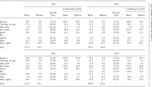
In Table 1, we have the basic household wealth holdings in the PSID 1984, 1989, 1994, and 1999. These are in constant 1993 dollars and include business equity.15 Median household wealth rises modestly over time from $45,200 in 1984 to $46,000 in 1989, to $49,100 in 1994 and to $56,800 in 1999. The home ownership rate rises from 59.6 percent in 1984 to 66.2 percent in 1999. During the same interval, condi-tional on owning, median equity falls from about $55,000 in the 1980s to about $50,000 in the 1990s. One reason for the equity decline may be the changing U.S. tax code. Interest deductions on household debt were eliminated by the early 1990s, except for mortgage debt. This tax change and the growth of convenient refinancing of home mortgages (Hurst and Stafford 2000) may account for declining equity in the 1990s. At the same time median vehicle equity rose some, reflecting the possibil-ity that—despite the rise in auto leasing—many families substituted vehicle financed auto purchases by refinancing their home mortgage, drawing equity from their home. At the same time that tax-deductible mortgage debt was rising, so too was nondeduct-ible noncollateralized debt (largely credit card carry over balances, along with debt for medical dental and educational services).

13. For example, consider a family physician who rents an office where she works. When asked the value of her business, she should correctly compute the discounted value of her future profits. However, when asked how much she could get if she sold her business, the amount would be trivial, since the profits come mostly from her human capital. Of course, the list of her patient names and her endorsement is of value to another doctor but this is still quite an illiquid asset.

l4. Nevertheless, we do include the value of nonowner-occupied and commercial real estate, which is also likely to be less liquid than financial wealth holdings.

(9)

330

The

Journal

of

Human

Resources

Table 1

U.S. Household Wealth, Panel Study of Income Dynamics (Thousands of 1993 U.S. dollars)

1984 1989

Conditional on Own Conditional on Own

Percent Percent

Mean Median Own Mean Median Mean Median Own Mean Median

Business 24.0 0.0 12.2% 196.2 56.3 27.8 0.0 13.4% 208.0 48.4

Checking savings 17.6 2.9 80.8% 21.8 5.8 21.5 3.0 81.2% 26.5 6.1

Other debt 2.6 0.0 46.3% 5.7 2.2 3.5 0.0 50.2% 7.0 3.0

Real estate 19.7 0.0 20.0% 98.6 36.1 28.1 0.0 19.6% 143.3 37.5

Stocks 10.3 0.0 24.8% 41.4 10.1 15.7 0.0 27.9% 56.3 12.1

IRA

Vehicle 8.0 4.3 83.2% 9.6 6.2 9.4 6.1 83.1% 11.4 7.3

Other 14.7 0.0 23.4% 63.0 4.6 7.1 0.0 26.3% 27.1 6.1

Home equity 41.7 19.5 59.6% 69.9 54.9 49.6 17.0 60.3% 82.3 54.5

Total 133.3 45.2 155.9 46.0

1994 1999

Business 22.0 0.0 13.2% 165.9 40.5 35.9 0.0 13.0% 277.0 36.0

Checking savings 19.3 3.0 77.8% 24.9 5.1 16.5 2.7 84.0% 19.7 4.1

Other debt 6.1 0.1 50.6% 12.0 4.6 4.9 0.0 47.0% 10.5 4.5

Real estate 24.0 0.0 17.7% 135.6 40.5 22.6 0.0 17.2% 131.8 46.8

Stocks 28.5 0.0 34.5% 82.6 20.3 37.2 0.0 28.5% 130.4 27.0

IRA 22.4 0.0 32.5% 69.0 22.5

Vehicle 10.8 6.6 85.4% 12.6 8.1 11.9 6.3 — — —

Other 9.5 0.0 24.5% 38.7 9.1 7.8 0.0 19.7% 39.8 9.0

Home equity 44.3 17.2 62.8% 70.7 48.6 50.5 22.5 66.2% 76.3 53.8

Total 152.3 49.1 199.9 56.8

(10)

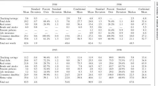
Over the period 1984–99, stock ownership (including equities in an Individual Retirement Accounts or IRAs) rose strongly, from 24.8 percent in 1984 to 27.9 percent in 1989 and then 34.5 percent in 1994. The PSID question sequence for 1999 separated IRAs from other stock owning. As of 1999, the direct stock ownership rate for families was 28.5 percent and 32.5 percent owned IRAs. At this point, we cannot identify those holding IRAs with some or all equities in them and who hold no non-IRA equities. However, a reasonable estimate of those with some stocks in either IRAs or otherwise holding stocks is probably in the 40–50 percent range as of 1999. Although the mean wealth in Sweden (Table 2) is only about half of that in the United States, the median wealth exceeds the U.S. median by the order of 10–20 percent. This demonstrates the much higher inequality and positive skewness of the U.S. wealth distribution. In both countries, the mean to median ratio has increased 1984–98/99, but much more in the United States. Measured in this way, inequality in wealth has thus increased more in the United States than in Sweden. These com-parisons suffer from the previously noted fact that assets in unincorporated business are included in the PSID but not in the HUS, and that more durables are included in the HUS than in the PSID. A more standardized comparison is offered below.

One of the most pronounced changes in Sweden seems to be the rise in real estate in the mid-late 1990s. The percentage of homeowners rose from about 60 percent in the 1980s and early 1990s to almost 70 percent (68.9 percent) in 1998, and a rising percentage of families held other real estate over the period 1984–98. It is also interesting to note that endowment policies and private pension policies have increased as a complement to Social Security and negotiated group pensions. Debts decreased after the major tax reform in 1991 when interest deductions became less favorable, but have increased at the end of the 1990s as the marginal tax rates again have become higher. Swedish households held more money in bank accounts follow-ing the tax reform, since the new tax system gives a more favorable treatment of interest earned on bank accounts than did the old system.

In the 1990s, more than 90 percent of Swedish families held a bank account. In the United States, the percent with a bank account first fell from 80.8 percent to 77.8 percent in 1989–94. Then, from this dip in 1994 the percent of families with a bank account rose back up to 84 percent in 1999. The significance of a substantial share of families with no bank accounts in the study of wealth ownership in the United States is that it fits into a larger pattern of wealth dispersion. That is, at the lower end of the U.S. wealth distribution a group of U.S. families is persistently ‘‘out of the financial game.’’ This group appears to differ from a growing negative wealth segment. This segment encompasses people who at one time had enough financial credibility to be eligible for credit, but whose financial position deteriorated into a situation of negative wealth. To consider this group in the United States and Sweden, we turn to the distribution of overall household (less business) wealth.

(11)

332

The

Journal

of

Human

Resources

Table 2

Swedish Household Wealth, Household Market and Nonmarket Activity Survey (Thousands of 1993 U.S. dollars)

1984 1986

Standard Percent Standard Conditional Standard Percent Standard Coditional Mean Deviation Own Deviation Median Mean Mean Deviation Own Deviation Median Mean

Checking/savings 5.8 0.3 — — 2.9 5.8 6.8 0.3 — — 2.5 6.8 Total debt 19.2 0.7 69.4% 1.3 7.8 27.7 24.8 1.3 76.4% 1.1 8.0 32.4 Real estate 9.0 0.8 24.9% 1.1 0.0 36.4 13.4 2.5 28.2% 1.1 0.0 47.3 Bonds and stocks 6.0 0.8 — — 0.1 6.0 5.5 0.6 — — 0.1 5.5 Pension policies — — — — — — 1.2 0.2 14.4% 0.9 0.0 8.2 Life insurance — — — — — — 0.9 0.1 14.2% 0.9 0.0 6.6 Consumer durables 25.1 0.6 100.0% 0.0 15.6 25.1 27.2 0.6 100.0% 0.0 16.0 27.2 Home value 35.8 1.3 61.2% 1.3 24.5 58.5 32.1 0.9 60.9% 1.2 21.1 52.7 Total net worth 62.6 1.9 48.4 62.4 3.1 48.3

1993 1998

Checking savings 11.2 0.4 96.6% 0.5 5.7 11.6 11.9 0.4 89.0 89.0% 5.8 13.4 Total debt 20.8 0.7 72.2% 1.2 8.8 28.7 25.5 0.8 73.5 73.5% 17.2 34.8 Real estate 21.8 3.9 28.7% 1.1 0.0 75.5 18.8 1.9 29.4 29.4% 0.0 63.9 Bonds and stocks 6.6 0.5 83.7% 1.0 0.1 7.8 14.5 0.7 63.7 63.7% 1.6 22.8 Pension policies 3.4 0.3 32.6% 1.2 0.0 10.5 2.8 0.2 24.9 24.9% 0.0 11.1 Life insurance 1.2 0.2 14.0% 0.9 0.0 8.3 3.5 0.3 29.4 29.4% 0.0 11.8 Consumer durables 24.9 0.6 99.9% 0.1 24.5 24.9 24.4 0.5 100.0 100.0% 22.3 24.4 Home value 35.4 1.3 59.1 1.3 22.0 59.8 40.6 1.1 68.9 68.9% 37.0 58.9

Total net 83.5 4.6 54.8 90.9 2.8 67.6

(12)

Klevmarken,

Lupton,

and

Stafford

333

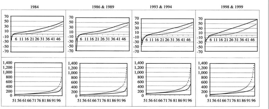
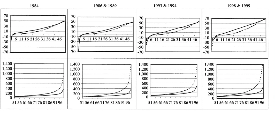
Figure 1

PSID and HUS Wealth Distribution

(13)

Table 3

Measures of Despersion in the PSID and HUS Household Wealth

1984 1986 & 1989 1993 & 1994 1998 & 1999

Dispersion HUS PSID HUS PSID HUS PSID HUS PSID

90/10 23.2 n.a 39.5 n.a. 49.0 n.a. 37.0 n.a. 75/25 5.0 20.6 5.3 23.3 5.0 22.8 4.5 30.8

60/40 1.9 2.8 1.7 3.0 1.7 2.9 1.7 3.0

PSID/HUS Ratio at Given Percentile

15th percentile 0.10 0.07 0.03 0.00

25th 0.32 0.34 0.28 0.20

40th 0.66 0.60 0.61 0.54

50th 0.83 0.84 0.82 0.73

60th 1.01 1.06 1.03 0.95

75th 1.34 1.50 1.27 1.35

90th 1.73 2.10 1.77 1.91

95th 2.13 2.63 2.05 2.45

99th 2.35 3.45 2.52 3.26

lies above the LH segment for the United States and that, after crossing the Swedish curve from below at somewhat above the median, the U.S. distribution rises steeply above the Swedish distribution. In brief, the U.S. wealth distribution is far more dispersed than that of Sweden. Further, while this dispersion has remained relatively constant in Sweden over the last two decades, it has grown substantially in the United States.

Both countries exhibit a negative household wealth segment. In the United States, this segment grows progressively larger and the (constant dollar) absolute values of the percentiles in this segment become progressively larger through time. In Swe-den, the negative wealth segment first grows, 1984–86, and then—after the tax re-form—it diminishes successively in 1993 and 1998.16_{Another difference in the two} countries is the large flat segment of U.S. households (but not for Swedish house-holds) that are essentially out of the asset game and have zero wealth by virtue of having neither assets nor liabilities.17_{For the United States, combining the negative} and zero wealth leads to positive wealth starting at the percentile teens.

The strong and growing relative dispersion of the U.S. household wealth can be seen in Table 3. As implied from our discussion of the low wealth segment of U.S.

16. Table 5 of the publicationFo¨rmo¨genshetsfo¨rdelningen i Sverige 1997 med en tillbakablick till1975. Report 2000:1, Statistics Sweden, O¨ rebro, Statistics Sweden, shows a completely different picture. From 1975 to 1997 the share of households with zero wealth decreased from 23.6 percent to 6.6 percent and the share of households with negative wealth increased from 7.6 percent to 23.7 percent. However, these estimates most likely reflect more changes in the self-assessment procedures rather than changes in the distribution of wealth.

(14)

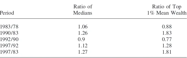
Table 4

Growth of Net Wealth in Sweden, Median & Top 1 Percent

Ratio of Ratio of Top

Period Medians 1% Mean Wealth

1983/78 1.06 0.88

1990/83 1.26 1.83

1992/90 0.9 0.77

1997/92 1.12 1.28

1997/83 1.27 1.81

Source:Fo¨rmo¨genhetsfo¨rdelningen i Sverige 1997 med en till-bakablick till1975, Report 2000:1, Statistics Sweden, O¨ rebro.

families, the 90/10 percentile ratio is not defined for the United States. For Sweden the 90/10 percentile ratio shows a peak in the beginning of the 1990s, but it may not be a robust statistic since the 10th_{percentile is also only a modest positive value.} Data on the very wealthy from Statistics Sweden suggest that the right end tail of the distribution has moved even further to the right in the period 1975–97 (see Table 4). The 75/25 percentile dispersion holds, however, pretty steadily at about five for Sweden, 1984–98. For the United States, it rises from 20.6 in 1984 and then to 23.3 in 1989 and then to 30.8 in 1999.

Comparing the PSID/HUS ratio by quantile is another way to assess the relative wealth dispersion in the two countries. For deciles at or below the median the PSID/ HUS ratio is always below unity and often radically below unity and drifts down over time. At the median, U.S. household wealth is a bit less than household wealth for Sweden and persists at about 10 percent less in the 1980s and the 1990s. For deciles above the median (60th_{and above) the PSID/HUS ratio is always above unity} and very substantially above unity in the upper quantile ranges and generally drifts upward over time. At the 95th_{percentile U.S. household wealth is about two to three} times as great as Swedish wealth.

For the United States, calculations of the mean wealth of the 400 richest families have been made using data from Forbes magazine (Broom and Shay 2000). As of 1984 (in 1999 dollars) the wealth of the 400 richest families averaged $504 million.18 By 1989, this had become $901 million, by 1994, it was $980 million, and by 1999, it had risen to an average of $2,590 million. This represents an increase from 1984 to 1999 of 5.14-fold. In the period 1994 to 1999 alone, the Forbes average rose by a factor of 2.6. From the PSID data at the 99th percentile, the growth was from $1.794 million in 1994 to $2.743 million in 1999. This is a far smaller growth factor (1.52) and is consistent with the claim of a rising dispersion in the U.S. household wealth distribution.

(15)

Using the tax authorities’ household definition, Statistics Sweden estimated that 522 households (the top 0.011 percent) had more than 31.3 million kronor taxable wealth in the end of 1997,19_{which approximates 2.9 million 1993 USD. This number} is much smaller than the U.S. mean estimate above for several reasons: It is not the mean wealth of the richest but a percentile measure of the lower bound and it is tax-assessed wealth and not total wealth. Nevertheless, it reflects that, even after adjusting for the size of countries, the wealthiest in Sweden are not as wealthy as the wealthiest in the United States. The wealth data of Statistics Sweden also permit a comparison of the growth rate of median household wealth with that of the top 1 percent. Table 4 gives the beginning and end period ratios of median wealth and the top 1 percent of wealth respectively, in constant prices.20_{For the 1983–97 period} as a whole the wealthiest have almost doubled their wealth while the median house-hold only got an increase of 27 percent. Inequality thus increased, although not as much as in the United States. Volatility was much higher among the wealthy than further down the wealth distribution, an indication of periods with decreasing in-equality.

One of the major factors accounting for the wide and growing difference between the United States and Sweden could be the low levels of wealth of African American families. Many African American families have virtually no household wealth. Rea-sons offered for these low wealth holdings include discrimination (Oliver and Sha-piro 1995; Conley 1998; Charles and Hurst 2000), and intergenerational transfer of asset holding knowledge (Chiteji and Stafford 2000). Another type of explana-tion looks at differential incentives for life-course accumulaexplana-tion of wealth in light of replacement ratios from Social Security in combination with bequest motives (Barsky, Bound, Charles, and Lupton 2000).

Taking African American wealth differences as a candidate factor in changing the shape of the overall U.S. wealth distribution, how different are the Swedish and United States wealth distributions if the African American difference within the United States is netted out? A simplistic way to net out this difference is to reexamine the U.S. wealth distribution excluding African American families. This is imple-mented in Figure 2.

The strong and growing relative dispersion of U.S. household wealth remains when restricting to white households only. This can be seen in the tabular summary of Figure 2 provided in Table 5. The 75/25-percentile ratio for white households rises from 13.3 (was 20.6 for the full sample in Table 5) in 1984 to 15.8 (was 23.3 for the full sample in Table 5) in 1989. The ratio stays about the same in 1994 (16.0) and 1999 (15.6). Again, comparing the PSID/HUS ratio by decile is another way to assess the relative wealth dispersion in the two countries. For deciles below the median the PSID/HUS ratio is somewhat greater but still always below unity and still often far below unity and drifts down over time. At the median U.S. household wealth is now a bit more than household wealth for Sweden and persists at about 5 percent more than the Swedish wealth in the 1980s and the 1990s. For deciles

19. Table 3 inFo¨rmo¨genshetsfo¨rdelningen i Sverige 1997 med en tillbakablick till1975. Report 2000:1, Statistics Sweden, O¨ rebro.

(16)

Klevmarken,

Lupton,

and

Stafford

337

Figure 2

PSID (White Households Only) and HUS Wealth Distribution

(17)

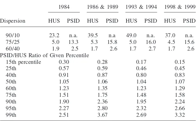
Table 5

Measures of Despersion in the PSID (White Households Only) and HUS Household Wealth

1984 1986 & 1989 1993 & 1994 1998 & 1999

Dispersion HUS PSID HUS PSID HUS PSID HUS PSID

90/10 23.2 n.a. 39.5 n.a 49.0 n.a. 37.0 n.a. 75/25 5.0 13.3 5.3 15.8 5.0 16.0 4.5 15.6

60/40 1.9 2.5 1.7 2.6 1.7 2.7 1.7 2.6

PSID/HUS Ratio of Given Percentile

15th percentile 0.30 0.28 0.17 0.15

25th 0.57 0.59 0.46 0.45

40th 0.91 0.87 0.80 0.83

50th 1.05 1.06 1.04 1.07

60th 1.23 1.35 1.23 1.29

75th 1.51 1.75 1.48 1.58

90th 1.90 2.36 1.95 2.24

95th 2.27 2.80 2.32 2.66

99th 2.51 3.67 2.69 3.32

above the median (60th_{and above), the PSID/HUS ratio is always above unity and} even more substantially above unity in the upper decile ranges and generally drifts upward over time. At the 95th _{percentile U.S. household wealth is a bit higher but} still in the range of two to three times as great as Swedish wealth. A simple explana-tion for this last relaexplana-tionship is that so few African American families are in the upper parts of the U.S. wealth distribution. To conclude, the greater ethnic heterogeneity of the U.S. population compared to the Swedish cannot explain the differences in wealth inequality.

(18)

from Table 2, one sees the same thing (1984: 1.29; 1986: 1.29; 1993: 1.52; 1998: 1.34).

We develop a parallel assessment of the macroeconomy for the United States. From 1986 to 1999, the private savings rate fell from the low teens to essentially zero. Much of the wealth gains were from rising equity prices and transferring assets into the equity markets in the late 1980s into the 1990s. These larger patterns and dispersion in the underlying rates of savings gave rise to growing wealth dispersion up until 2000 in the United States. The rate of U.S. wealth dispersion may have slowed or even decreased, at least since 2001, owing in part to the downturn in financial markets as well as to the increased exposure to higher returning assets for many new households.

Underlying explanations for differences in the wealth distributions can be found in the major differences in public policy in the two countries. As discussed in the introduction, the universal Swedish coverage of both basic and income-related public pensions since the beginning of the 1960s supplemented by occupational group pen-sions of wide coverage contrast with the employer-related group and private penpen-sions in the United States. So, too, do the differences in the magnitude of the public benefits that in Sweden include sickness benefits, maternity benefits, unemployment compen-sation, almost free medical care, and publicly provided care for the elderly. These benefits are universally guaranteed in Sweden not only for the poor but for the entire population. These public policy factors reduce the need for wealth in Sweden relative to the United States and are no doubt a major explanation for the lower degree of wealth inequality across households.

In addition to differences in social welfare policies, the Swedish income tax be-comes more progressive at lower inbe-comes than the U.S. income tax and until 1991 there was a joint progressive taxation of both labor and capital income. After 1991 in Sweden, capital income has been taxed at a flat rate roughly similar to the United States. However, there still remains in Sweden a real estate tax and a progressive wealth tax. The result of a larger guaranteed social safety net in addition to a more egalitarian tax policy in Sweden reduces both the need to accumulate assets for a rainy day as well as the incentives to accumulate wealth. It is this issue of accumula-tion and the mobility of wealth over time to which we now turn.

III. The Mobility of Household Wealth Holdings in

Sweden and the United States

(19)

plan? Another source of rising wealth inequality and differential mobility is long-term compositional changes in households. If a large share of the population moves into their peak preretirement earnings years, lifecycle theory would predict that they would have rapid wealth accumulation, possibly from a substantial mid-career base. If at the same time more newly formed young households take on debt from the older generations and have little home equity, household wealth dispersion will grow, but not necessarily in a full, life-course context.

To no small extent, if point-in-time inequality is the ‘‘stick’’ of capitalism then mobility is the ‘‘carrot.’’ While finding oneself at the lower tail of the wealth distribu-tion is wrought with all the discomforts of poverty, a belief in the possibility of upward mobility fills one with a certain amount of hope.21_{But the concept of mobility} is elusive. While mobility is by its nature a relative construct, it is not clear to what it must relate. For instance, consider an increase in wealth by a given proportion to all individuals. Provided that all individuals have at least some wealth (a strong assumption), this could be seen as a tremendous amount of mobility. But this is mobility related only to the individual at different points in time.

On the other hand, supposing that all individuals were the same in every respect except for their initial endowment of wealth, then quantile mobility would be nonex-istent given a proportionate increase in all wealth. That is to say that mobility in the sense of movement among the ranking of the population would be unchanged since an increasing monotonic transformation does not alter ordinal properties. Further-more, point-in-time absolute inequality would increase. Thus, a proportional increase in wealth, while certainly increasing individual mobility, has no effect on quantile mobility and leads to increased point-in-time inequality.22 _{Nevertheless, the belief} in a rising tide that raises all boats has dominated social and economic policy in the United States. In contrast, redistribution has been the focus of economic and social policy in some Northern European countries, particularly in the Nordic countries. This transatlantic difference in values and policy might be a major explanation of the great differences we have observed in wealth inequality between Sweden and the United States. However, despite these differences in cross-sectional inequality, it is not obvious how wealth mobility may differ between the two countries.

A thorough discussion of the roots of rank, or quantile, mobility is beyond the scope of this paper but some remarks are warranted. Quantile mobility in wealth is largely a result of behavior and initial heterogeneity as well as variable returns on investments. There are differences in the desires to postpone current for future con-sumption, the willingness to accept investment risks in exchange for higher returns, the amount of investment in human capital and hence the return to human wealth and the levels of investment in one’s progeny. In addition, simple differences in life-cycle stages is also a fundamental cause of variation and hence mobility. While today’s young and middle-aged households rest in the respective bottom and top of the wealth distribution, this will certainly reverse itself over the following 30 years,

21. This point is consistent with the wide political support in the United States for an elimination of the estate tax.

(20)

as the young become middle-aged and middle-aged consume their wealth in retire-ment. On the other hand, variation can also be a result of phenomena exogenous to individual choice. These range from various forms of discrimination that alter the ‘‘rules of game’’ for specific groups of people to inherent differences in ability. Distinguishing between tastes and inherent impediments is a crucial step in monitor-ing economic inequality.

While in both countries there is a variety of interesting assessments of macroeco-nomic factors, in this paper, we instead focus on a reduced form version of quantile mobility and examine the extent to which initial conditions affect quantile mobility without seriously ferreting out its fundamental causes. High wealth mobility (in dol-lars) can contribute to a high wealth inequality, and a high mobility might make a high inequality more acceptable from an equity point of view. We thus turn to a comparative analysis of mobility.

A. Background and Measures

How does mobility in the wealth distribution compare across the two countries? If the cross-sectional wealth distribution is widely dispersed is it still possible that the rich and poor trade places frequently in either or both countries? What do we mean by trading places? One definition is movement in relative position in the wealth distribution through time, such as changing location in the decile or quintiles of wealth through time. For comparison purposes we will rely primarily on wealth quintiles for the two countries. This is to avoid excessive detail in the mobility tables and because the sample sizes in HUS are not large enough for additional quantile disaggregation. The extent of wealth transitions across quantiles can be measured by Shorrocks’ index.23_{It measures the share of the off-diagonal elements in quantile} transition tables, such as Tables 6 through 9 below, and it ranges from zero (no mobility) to a value just above one (no stability). It is not invariant to the choice of quantiles and it will of course depend on the time span used. Factors that influence these transition tables were discussed in the introduction.

B. Measuring Mobility

For Sweden over the nine-year period, 1983/84–1992/93, the Shorrocks’ index for household decile wealth mobility has been estimated as 0.87 (Bager-Sjo¨gren and Klevmarken 1996), compared with the 0.804 for the United States over the ten-year period, 1984–94 (Hurts, Luoh, and Stafford 1998). For the United States between 1984–89 and then 1989–94, the Shorrocks’ measure rose modestly from 0.733 to 0.754 (Hurst, Luoh, and Stafford 1998). Looking at the period 1993–98 for Sweden, the HUS data for quintiles show a value of 0.744 for the Shorrocks’ index and for the PSID, 1994–99 the data for quintiles show a value of 0.592. These estimates are based on the transition matrices in Tables 6 and 7. While these measures suggest more wealth mobility in Sweden, it should be remembered that they are measures of

(21)

Table 6

Quintile Wealth Transition matrix for the United States 1994–99 (quintiles in 1993 USD)

Bottom Bracket 1 2 3 4 5

Quintile Value 2,949 29,730 80,752 206,195

1 0.583 0.273 0.099 0.031 0.015

2 1,043 0.267 0.435 0.223 0.058 0.016

3 22,011 0.087 0.208 0.419 0.232 0.055

4 66,118 0.048 0.079 0.193 0.481 0.2

5 165,345 0.014 0.022 0.051 0.2 0.713

Note: Shorrocks index of mobility equal to 0.592. Row numbers are 1994 quintiles while column numbers are 1999 quintiles. Bottom of quintile brackets reported adjacent to quintile numbers. Number of house-holds is 4,383.

mobility across quintiles (deciles in the previously cited research). If these quintiles themselves are wider apart and widening through time as shown for the United States, one cannot straightforwardly conclude that there is more wealth mobility in Sweden. Remembering that the absolute spread of the U.S. wealth distribution has been rising, it seems safe to conclude that wealth mobility is rising in the United States, a finding parallel to rising income mobility (Gottschalk and Moffitt 1994).

Much of the quintile wealth mobility is in the mid-range quantiles. The top and bottom quantiles are characterized by substantial persistence, partly the simple con-sequence of only single direction movement at the top and bottom quintiles. Of the families in the top U.S. wealth quintile in 1994, almost three-quarters (71.3 percent) are in the top quintile in 1999. Even in terms of deciles and extending the transition period to 10 years, between 1984 and 1994, for example, over half (53.3 percent)

Table 7

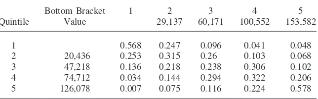
Quintile Wealth Transition matrix for Sweden 1993–98 (quintiles in 1993 USD)

Bottom Bracket 1 2 3 4 5

Quintile Value 29,137 60,171 100,552 153,582

1 0.568 0.247 0.096 0.041 0.048

2 20,436 0.253 0.315 0.26 0.103 0.068

3 47,218 0.136 0.218 0.238 0.306 0.102

4 74,712 0.034 0.144 0.294 0.322 0.206

5 126,078 0.007 0.075 0.116 0.224 0.578

(22)

of those initially in the top decile were still in the top decile.24_{For Sweden, of the} families in the top quintile in 1993 almost three-fifths (57.8 percent) remained in the top quintile in 1998. At the other end of the spectrum, of those U.S. families in the bottom decile in 1984—which include numerous negative wealth families— about half are still in the bottom decile in 1989 and about two-fifths are in the bottom decile a decade later in 1994. This is more important when we remember that the 1994 bottom decile for the United States was in much greater negative territory than the 1984 bottom decile (See Figure 1).

For 1994 to 1999, Table 6 shows that 58 percent or almost three-fifths of U.S. families in the lowest quintile in 1994 were still in the lowest quintile in 1999. For Sweden (Table 7), of those in the bottom quintile in 1993, more than half (56.8 percent) were in the bottom quintile in 1998. Of course, absolute numbers matter, since the real value of assets of those in the bottom quintile in Sweden is well above the assets of those in the bottom quintile in the United States

There are families with persistently low and negative wealth in the United States, despite the overall drift toward greater wealth mobility. In the mid-quintiles, since movements can occur both upward and downward from the initial position, there is less persistence. Using the overall summary of the Shorrocks’ index, we have a five-year quintile-based value of 0.744 for Sweden (1993–98) and 0.592 for the United States (1994–99), indicating a higher degree of mobility in Sweden than in the United States on the order of 25.7 percent.

C. Standardizing Mobility Differences

Although the quintile mobility gap between Sweden and the United States is large, we can attribute much of this to differences in the demographic composition of the two countries. There is a significant wealth gap between African Americans and their compliment. In addition, lifecycle theory suggests hump-wealth age profiles, which have implications for aggregate wealth mobility. These effects on wealth accu-mulation are magnified under a model of heterogeneous agents acting under various forms of risk. For instance, consider households that act as buffer-stock savers in the sense of Deaton (1991) or Carroll (1997) in the early portions of their lives but then as standard lifecycle hypothesis consumers from age 40 onward.25_{In this case,} since most young households accumulate very little wealth, quintile mobility is pri-marily a result of income and returns shocks that affect the optimal buffer stock of wealth. On the other hand, as households move into their prime savings years, the heterogeneity of behavior combined with increasing income lead to more quintile mobility. Finally, post-retirement heterogeneity of behavior with regard to bequests, life expectancy and rates of return combine with large and falling levels of wealth, which all lead to even higher levels of mobility. This story is borne out in the quintile transition tables portrayed in Table 8 which reflect mobility in the United States between 1994 and 1999 for three age groups: less than 40, 40 to 65, and older than

24. See Hurst, Luoh, and Stafford (1998). Remember that the families who are still intact over a 10-year span are overrepresentative of stable families.

(23)

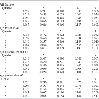
Table 8

Total U.S. Household Wealth Transition Tables by Quintiles (PSID): 1994 to 1999

Full Sample

Quintile 1 2 3 4 5

1 0.592 0.291 0.080 0.031 0.006

2 0.219 0.459 0.233 0.062 0.026

3 0.092 0.167 0.445 0.242 0.053

4 0.048 0.056 0.183 0.480 0.223

5 0.035 0.026 0.060 0.187 0.692

Age less than 40

Quintile 1 2 3 4 5

1 0.754 0.172 0.022 0.020 0.032

2 0.292 0.460 0.186 0.038 0.024

3 0.119 0.257 0.466 0.149 0.010

4 0.064 0.034 0.221 0.532 0.149

5 0.028 0.013 0.039 0.181 0.738

Age between 40 and 65

Quintile 1 2 3 4 5

1 0.549 0.307 0.090 0.048 0.007

2 0.236 0.470 0.221 0.041 0.032

3 0.064 0.146 0.495 0.247 0.048

4 0.042 0.059 0.165 0.505 0.228

5 0.028 0.020 0.043 0.188 0.721

Age greater than 65

Quintile 1 2 3 4 5

1 0.593 0.296 0.081 0.027 0.003

2 0.204 0.455 0.244 0.074 0.023

3 0.113 0.158 0.385 0.271 0.074

4 0.083 0.067 0.190 0.392 0.269

5 0.072 0.068 0.154 0.188 0.517

Note: Shorrocks index of mobility for the full sample equal to 0.583, 0.512 households with head age less than 40, 0.565 for households with head age between 40 and 65, .0664 for household heads age greater than 65. Household wealth includes private business equity.

65. As suggested, the Shorrocks’ index increases over the life cycle by 10 percent from the first to the second age group and then by 17 percent from the second age group to the oldest. The point here is that these lifecycle characteristics as well as other various demographic features of Sweden and the United States can be contribu-tors to the large mobility gap between the two countries, provided that there are differences in this respect.

(24)

plans, individual retirement accounts, or privately held assets, across all age groups should lead to an increase in quintile mobility, given heterogeneous portfolio compo-sitions combined with varying rates of return. Nevertheless, these channels for in-creased mobility are likely to be most prevalent and increasing for older age groups. Indeed, we find that while the Shorrocks’ index has fallen for the youngest age group (younger than 40) from 0.535 to 0.512, the index has increased by 11.7 percent for households aged 40 to 65 and by 10.9 percent for households older than age 65.26 Given this rise in the heterogeneous volatility of wealth evolution for those older than age 65, proposed policy measures to increase individual access and hence exposure to the corporate equities market by way of individualized Social Security accounts, while increasing mean returns, is likely to also further increase rate of return hetero-geneity and hence wealth inequality.

Although age and other demographic differences may be important, the largest difference between Sweden and the United States is in the initial wealth distribution. As shown in Table 3, the United States wealth distribution is much more spread out than the Swedish distribution. The result is that the quintiles from which we are measuring mobility are larger and hence a larger absolute change in wealth is re-quired in order to change quintiles. It is therefore difficult to compare mobility in the two countries. Given the larger wealth dispersion, it is possible for the United States to have larger absolute wealth changes but still have less rank mobility.

In the next section, we standardize the initial wealth distribution between Sweden and the United States and recompute the transition tables. We also outline a method for standardizing (or matching) on multiple variables. We apply this matching method to the HUS-PSID data to see if there is differential wealth mobility beyond that related to the cross-sectional dispersion and factors such as race, age, marital status, and longer run family income.

IV. Cross-National Transitions in a Multivariate

Matching Context

Consider a U.S. 1994 household distribution created by matching to the (almost) same year (1993) for Sweden. Going forward from that point, and an-chored at the sameabsolutestarting point, would we observe the same relative wealth mobility? Table 9 presents such a matched quintile transition matrix for the PSID, 1994–99. On inspection, the matching moves a majority of the individual elements closer to the corresponding HUS elements in most cases, particularly in the upper quintiles. As a result, the Shorrocks’ index of this matched transition matrix becomes 0.661, up from the baseline of 0.592 and much closer to the 1993–98 HUS value of 0.744.

Is it the case that additional matching on basic economic and demographic vari-ables can further align the quantile mobility in the two countries? That is, we can

(25)

Table 9

Matched Wealth Transition Mtarix for the United States 1994–99 (quintiles in 1993 USD)

Quintile 1 2 3 4 5

Bottom Bracket

Value 18,006 47,521 97,200 181,308

1 0.603 0.253 0.089 0.027 0.027

2 20,445 0.164 0.431 0.253 0.11 0.041

3 47,272 0.102 0.218 0.374 0.218 0.088

4 74,718 0.089 0.048 0.226 0.37 0.267

5 126,174 0.041 0.048 0.061 0.272 0.578

Note: Shorrocks index of mobility equal to 0.661. Row numbers are 1994 quintiles while column numbers are 1999 quintiles. Bottom of quintile brackets reported adjacent to quintile numbers. Number of house-holds is 732.

explain part of the difference in relative mobility by considering the distinct wealth-holding patterns of African Americans. Some of the difference reflects the basic differences in wealth dispersion. If we add lifecycle factors such as age, marital status, and children, do relative wealth mobility differences persist?

A. The Matching Methodology

The general aim of matching is to obtain a sample of PSID observations, which is as close as possible to the HUS sample. We use the matching technique outlined in Rubin (1979). We begin with two samples: the PSID (S1) withN1observations and the HUS (S2) withN2observations whereN1⬎N2. We consider a set of matching variables that include wealth, income, and various demographicsxij∈Sjj⫽1, 2; i⫽1, 2, . . . ,Njwherexijis a 1⫻pvector of matching variables for each individual. The criterion for a close match between two observations is the Mahalanobis metric. This metric is a weighted measure of squared deviations where the weight, as sug-gested by Rubin (1979), is the pooled empirical covariance matrix:

(1) ZRubin⬅[(X′1X1⫺N1X¯′1X¯1)⫹(X′2X2⫺N2X¯′2X¯2)]/(N1⫹N2⫺2)

Then, after randomly sorting the HUS data, matches from the PSID are chosen according to the following algorithm:

s11⫽arg min s1i∈S1

(x21⫺x1i)z⫺1₍_x21

⫺x1i)

(2) s12⫽arg min s1i∈(S1⫺s11)

(x22⫺x1i)z⫺1₍_x 22⫺x1i)

s13⫽ arg min s1i∈(S1⫺s11⫺s12)

(x23⫺x1i)z⫺1₍_x23

⫺x23⫺x1i)

(26)

Note that the suggestion ofzRubinshould work well if the two data sets (HUS and PSID) have approximately the same covariance matrix. But if they differ in covari-ance the larger data set (PSID) will dominate in the estimate ofZand we will tend not to get as close a match of PSID observations to HUS. For this reason matching has also been done with a covariance matrix only estimated from HUS-data,

(3) zhus⬅[(X′2X2⫺N2X¯′2X¯2)]/(N2⫺1)

For every observation in the HUS sample the closest match among the PSID obser-vations was searched using the above matching, algorithm. Matching was done with-out replacement, so when a PSID match was found this observation was no no longer eligible in the following searches. This implies that the search order could become important. Rubin thus suggested that the mother data set (HUS) should be sorted randomly before the search starts. In our case the PSID sample is more than four times the size of the HUS sample and the order of the HUS sample did not seem to be very important to the results. Matching with replacement only gave a margin-ally closer match.

In addition to matching on the 1993–94 household wealth in 1993 USD, matching was done on the following variables: number of adults in the household, number of children in the household, age of head, schooling of head, marital status of head and household disposable income as of 1993. We also conducted matching separately for whites and in a few cases by family type (single with/without children, couples with/without children).

B. Matching Results

We summarize the results in Table 10. In the first half of the table there are results from matching on the entire PSID sample independently of race, while in the second half only white households were used. The very first rows give the median wealth and the ratio of the fourth to the first quartile for the HUS samples in 1993 and 1998 followed by Shorrocks’ mobility measure. Then follows the corresponding statistics for the PSID. These are the numbers to which the statistics for the matched samples should be compared.

We obtained the closest match and the highest mobility when we matched only on the 1993–94 household wealth. Adding other variables to the matching criterion resulted in a matched wealth distribution, which deviated more from the HUS distri-bution and the corresponding mobility measure became smaller. Similarly, when we matched by family type, which implies that the search became more limited, the matched distribution deviated more from the HUS distribution and the matched tran-sition matrix had a lower mobility, compared with a match using only the 1993– 94 household wealth. Limiting the sample to whites actually lowered observed mo-bility from 0.592 to 0.585, while matching on whites only increased the matched mobility measure marginally—from 0.661 to 0.698. Although there is a small differ-ence in mobility between whites and nonwhites, this heterogeneity in the U.S. popu-lation cannot explain the difference between Sweden and the United States in mo-bility.

(27)

Table 10

Wealth mobility 1993/4 to 1998/9 in Sweden and the United States

Match With Distance Median Shorrock’s Dataset/Experiment variables Replacement measure wealth Q4/Q1 mobility

HUS 1993 61,583 6.17

HUS 1998 77,217 5.27

HUS 93–98 0.744

PSID 1994 39,818 158.52

PSID 1999 52,603 69.92

PSID 94–99 0.592

PSID Match94 nw93/94 no 61,548 6.17

PSID Match99 nw93/94 no 71,928 10.07

PSID Match94/99 0.661

PSID match94 all no zrubin 84,498 19.71

PSID match99 all no zrubin 124,676 17.43

PSID match94–99 0.581

PSID match94 all no zhus 41,727 33.72

PSID match99 all no zhus 69,531 23.92

PSID matcg94–99 0.675

PSID White94 71,458 24.9

PSID White99 93,027 18.87

PSID White94–99 0.585

PSID White match94 nw93/94 no 61,548 6.14

PSID White match99 nw93/94 no 78,641 9.49

PSID White match94–99 0.698

PSID White by family match94 nw93/94 no 59,461 7.5 PSID White by family match99 nw93/94 no 78,881 11.19

PSID White by family match94–99 0.688

PSID White match94 all no zrubin 89,714 15.81 PSID White match99 all no zrubin 132,348 13.72

PSID White match94 all no zhus 49,029 18.63

PSID White match99 all no zhus 79,888 16.46

PSID White match94 all but nw no zrubin 137,700 14.9 PSID White match99 all but nw no zrubin 185,096 14.06

PSID White match94 all but nw no zhus 135,614 15.52 PSID White match99 all but nw no zhus 174,546 14.45

(28)

much closer to the original PSID sample and they give mobility measures, which are almost as low as the observed measure. Differences in income and in demograph-ics do not seem to explain the difference between the two countries either. One can conclude from these exercises that while differences in income and demographics between Sweden and the United States may have some effect, differences in the initial wealth distribution account for a majority of differences in mobility. Nonethe-less, this could simply imply that initial wealth is a sufficient statistic for all other differences when examining mobility, and not that these other variables are incre-mentally unimportant.

Thus, the most important element of standardization in comparing Swedish and United States mobility measures is apparently to match on 1993–94 household wealth. The observation that the Swedish distribution of wealth is less dispersed than in the United States suggests selecting most of the observations from the middle of the U.S. distribution. The quintiles of this matched 1999 distribution will thus not be as wide as the quintiles of the 1999 original distribution, and therefore mobility will increase. Table 9 shows, however, that the fourth to first quintile ratio of the 1999 matched distribution is about twice as high as the quintile ratio of the 1998 Swedish distribution, and thus the matched mobility measure reaches only about halfway toward the Swedish mobility measure.

Table 11 compares the 1993/94–1998/99 dollar changes in household wealth for the two countries. The median change in Sweden was almost $12,000, about twice as much as in the United States. However, the mean change was almost three times as high in the United States as in Sweden ($45,569 versus $16,425). The U.S. distri-bution of change was thus much more positively skewed than the Swedish. The U.S. dispersion is more than four times the Swedish dispersion, and has a higher differ-ence between the ninth and the first deciles. Limiting the U.S. population to whites does not decrease the dispersion of the change in wealth; on the contrary, the standard deviation increases by more than 20 percent and the decile range by more than 30 percent. Moreover, after matching on the 1993–94 household wealth most of these differences remained. These results suggest that dollar mobility is higher in the United States than in Sweden, while (relative) quantile mobility is higher in Sweden. We have so far used the Swedish measure of mobility as a reference, but it is probably inflated. The reason is that there is a fair amount of randomness from

impu-Table 11

1993/94–1998/99 change in net wealth; descriptive statistics (Thousands of 1993 USD)

Data set Nobs Mean Std.err. Median D9-D1 Max

HUS 1993–98 732 16.4 124.9 11.8 150.7 1,532.8 PSID 1994–99 4,383 45.6 525.0 6.0 216.2 23,803.6 PSID 1994–99, whites 2,921 57.6 640.2 14.0 286.1 23,803.6 PSID match 1994–99 732 36.0 136.6 9.9 200.4 1,485.1