(Case Study : Boyolali Regency)
THESIS
Oleh :
Constantina Ajeng Widi P.
NIM : 972011007
Program Studi Magister Sistem Informasi
Fakultas Teknologi Informasi
Universitas Kristen Satya Wacana
Salatiga
PRAKATA
Puji syukur kepada Tuhan Yesus Kristus yang telah menyatakan kasih karunia-Nya,
sehingga penulis mampu menyelesaikan Thesis yang berjudul “Identification of Spatial
Patterns of Food Insecurity Region
s Using Moran’s I (Case Study :
Boyolali
Regency)”.
Laporan thesis ini disusun guna memenuhi persyaratan untuk memperoleh gelar
Master of
Computer Science
(M.Cs.) pada Program Studi Magister Sistem Informasi Fakultas
Teknologi Informasi Universitas Kristen Satya Wacana Salatiga.
Dalam menyelesaikan thesis ini, penulis tidak lepas dari dukungan berbagai pihak.
Oleh karena itu, dengan segala kerendahan hati penulis ingin mengucapkan banyak terima
kasih kepada :
1.
Bapak Dr
.
Dharmaputra Palekahelu
,
M.Pd selaku Dekan Fakultas Teknologi
Informasi Universitas Kristen Satya Wacana Salatiga.
2.
Bapak Prof. Dr. Ir. Eko Sediyono
,
M.Kom selaku Kaprogdi Magister Sistem
Informasi Universitas Kristen Satya Wacana Salatiga
3.
Bapak Dr. Ir. Wiranto Herry Utomo, M.Kom., selaku pembimbing pertama
yang telah membantu penulis dari awal hingga akhir penyelesaian tugas akhir
ini
4.
Bapak Sri Yulianto J. P., S.Si., M.Kom., selaku pembimbing kedua yang telah
banyak memberikan bantuan dan nasehat kepada penulis.
5.
Staff pengajar, Tata Usaha dan Karyawan Fakultas Teknologi Informasi.
Terimakasih atas kuliah dan kerjasama yang diberikan selama ini. Terima
kasih untuk semua bantuannya.
6.
Bapak dan Ibu, kakak, adik, dan seluruh keluarga yang banyak memberikan
doa dan dukungan selama menyelesaikan tugas akhir ini.
8.
Teman-teman MSI angkatan 08 yang telah banyak membantu penulis dalam
menyelesaikan studi S2.
Penulis menyadari bahwa laporan ini sangat jauh dari kesempurnaan, sehingga
merupakan suatu kehormatan bila penulis menerima kritik dan saran untuk penelitian ini.
Akhir kata, kiranya Thesis ini dapat memberikan manfaat baik bagi penulis sendiri, bagi
Fakultas Teknologi Informasi UKSW Salatiga, maupun bagi pihak-pihak yang membaca
tulisan ini.
Salatiga, Juni 2013
Daftar Isi
Halaman
Halaman Judul ... i
Halaman Pengesahan ...
ii
Halaman Pernyataan ...
iii
Prakata ...
iv
Daftar Isi ... vi
Daftar Gambar ...
vii
Daftar Tabel ...
viii
Abstract
...
ix
Bab 1
Introduction ...
1
Bab 2
Literature Review ...
2
2.1 Research Preview ...
2
2.2 Eksploratory Spatial Data Analysis (ESDA) ...
3
2.3 Spatial Autocorrelation ...
3
2.4 Moran’s I
...
3
2.5 Food Insecurity ...
4
Bab 3
Metodology Research ...
5
3.1 Stages of Research ...
5
3.4 Desain and Architecture Model ...
5
Bab 4
Result ...
6
Bab 5
Conclusion ...
9
Daftar Gambar
Halaman
Figure 1
Percentage of the underprivileged population in Boyolali
Regency ...
2
Figure 2
Spatial Cntiguity Matrix ...
3
Figure 3
Desain and Architecture Model ...
5
Figure 4
Queen Contiguity Matrix...
6
Figure 5
Underprivileged population in 2008 ...
7
Figure 6
Underprivileged population in 2009-2010 ...
7
Figure 7
Households without access to electricity in 2008 ...
7
Figure 8
Households without access to electricity in 2009-2010 ...
8
Figure 9
LISA map 2008 ...
8
Daftar Tabel
Halaman
Table 1
Spatial patterns of Moran’s I
...
4
Table 2
Food insecurity indicators ...
4
Table 3
Calculation of GISA ...
6
Identification of Spatial Patterns of Food Insecurity
Regions Using Moran's I (Case Study: Boyolali Regency)
Constantina A. Widi P.
Faculty of InformationTechnology Satya Wacana Christian
University
Diponegoro Street, 52-60 Salatiga 50711, Indonesia
[email protected]
Wiranto Herry Utomo
Faculty of InformationTechnology Satya Wacana Christian
University
Diponegoro Street, 52-60 Salatiga 50711, Indonesia
Sri Yulianto J. P.
Faculty of InformationTechnology Satya Wacana Christian
University Diponegoro Street, 52-60 Salatiga 50711, Indonesia
1.
INTRODUCTION
Boyolali Regency is one area of rice production surplus in 2008. However, some sub-districts in Boyolali Regency, such as sub-district Juwangi, Wonosegoro, Karanggede, Klego and Selo threatened with food insecurity [1]. Food insecurity can be defined as a condition in which individuals or households that do not have access to the economy (insufficient income), do not have physical access to obtain sufficient food, to a normal, healthy and productive life, both in quality and quantity [2]. One indicator of food insecurity is a percentage of underprivileged population. If an area has a percentage of underprivileged population of more than 25%, then the area is said to be food insecurity [3]. Figure 1 shows the percentage of underprivileged population from 2008-2010 in Boyolali Regency based on BPS [4]. Numbers on the X-axis represents a district in Boyolali Regency, and the numbers on the Y axis is the percentage of underprivileged population. Based on Figure 1, there are 16 districts that have a percentage of underprivileged population of more than 25% in 2008. This suggests that the level of food insecurity in Boyolali Regency is big enough.
Figure 1 Percentage of the underprivileged population in Boyolali Regency Regency Up to now, the measurement results of food insecurity area, are displayed in the form of maps, but there are still some weaknesses, such as maps that are still not able to give an overview of the factors that cause the occurrence of food insecurity in the area and not yet illustrate the dynamics of incident in the spatial pattern based on neighbors analysis.
Exploratory spatial data analysis (ESDA) is part of the process of exploration and data analysis (EDA) [5]. One of the goals ESDA methods, among others, is to detect spatial patterns appear in the data set (cluster, random, dispersed) [6]. Spatial Autocorrelation (SA) is part of the ESDA. One of the dimensions of SA is neighborhood and distance [5]. Moran's I is one of the oldest indicators of spatial autocorrelation [7].
2.
LITERATURE REVIEW
2.1
Research Preview
Indonesian government in cooperation with the World Food Program (WFP) has compiled a map of food insecurity that is a tool to determine regions with food insecurity issues and the underlying the incidence of food insecurity that would be used as a policy for overcoming food insecurity [9]. In the Map of Food Security and Vulnerability Atlas (FSVA) uses seven indicators of food insecurity. Composite map of food insecurity is resulted from the combination of all indicators of chronic food insecurity by using a weighting, based on the percentage of each indicator of food insecurity. [9] In FSVA developed the concept of food security, based on the three dimensions of food security (availability, access and utilization of food) in all conditions not only on food insecurity situation. The second consideration, FSVA also intended to determine the true causes of food insecurity or in other words, vulnerability to experience food insecurity, not only food insecurity itself [2].
Research on spatial data analysis has also been done by Prasetyo. That study aimed to compare the methods of analysis and mapping of endemic outbreaks of brown plant hopper on basic commodities and horticultural plants uses spatial autocorrelation method. Gisa, LISA, and brittle Ord Statistic used in modeling BPH endemic. Results of this study indicate that the pattern of hotspots in 37 districts in the area and pattern coldspots in 13 districts from 2001 to 2010 can be classified using this method. From the comparison of local Moran experiment frail Ord maps of BPH experiment in 2001, 2006 and 2010, found that the indications on the hotspot on local Moran is the same as an indication of Getis Ord grouping based on the value of Z (Gi)> 2 [10].
Another study also conducted by Tsai PJ. Goal of this study was to detect changes in the spatial patterns of clusters of health problems and risk factors among women and men using Moran's I and logistic regression in Taiwan. In the distribution analysis uses medical cases from the Taiwan National Health Insurance (NHI), and the mid-year population average, then applied to the global and local Moran test. Meanwhile, the logistic regression model was used to test the characteristics of similarities and differences between men and women and formulate risk factors. Results of this study showed that the geographic distribution of the cluster in which neoplasms commonly found to relate closely with
the location in arseniasis-endemic areas in Southwest and Northeast Taiwan, and locations in urban regions (for women) and cluster in Changhua and Yunlin (for men). High population density in urban regions show clusters of carcinogens in 3 major urban centers in Taiwan (ie, Taipei, Taichung, and Kaohsiung) for women neoplasms. From this study it can be concluded that the cluster mapping may help to clarify issues such as spatial aspects of health issues. This information is helpful in assessing the spatial risk factors, which can assist in the implementation of effective health services [11].
In this study, Moran's I is used to identify the spatial pattern of regional food insecuritys in 2008-2010 and determine whether an indicator that influences food insecurity in a district has a correlation with other districts.
2.2
Eksploratory
Spatial
Data
analysis
The aim of eksploratory spatial data analysis (ESDA) method is to detect the spatial method which is shown from assemblage data (cluster, random, dispersed). To detect the error possibilities in the data, to formulate the hypothesis based on spatial and geography method and to analyze the spatial model [6]. From the spatial concept, ESDA can be divided into 4 groups, spatial visualization distribution, spatial visualization association, local indicator spatial association (LISA), and multivariate indicators of spatial association [5].
2.2
Spatial Autocorrelation
Spatial Autocorrelation (SA) can be divided into two dimensions; the first dimension divides SA into neighborhood and distance. Neighborhood approach usually requires the standardization of spatial objects in the surrounding structure by determining the topology and weighting each data of observation result. The term distance means that the distance indicator is calculated from a spatial object towards its partner spatial object. The second dimension divides SA into global and local association. Global used to assess spatial interactions in the data. While the local association used to assess patterns of association around individuals and see how far the global pattern is reflected in the whole observed population [5].
One of the stages in SA is to build weight matrix of spatial objects. Prior to forming the weight matrix of spatial objects, there must be calculation of spatial contiguity matrix.
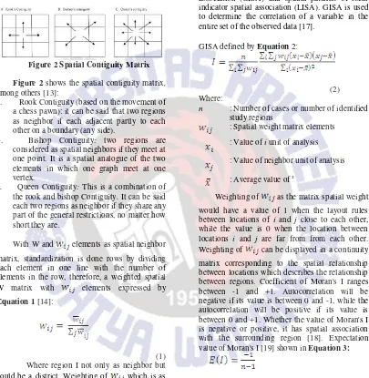
Figure 2Spatial Contiguity Matrix Figure 2 shows the spatial contiguity matrix, among others [13]:
a. Rook Contiguity (based on the movement of a chess pawn): it can be said that two regions as neighbor if each adjacent partly to each other on a boundary (any side).
b. Bishop Contiguity: two regions are considered as spatial neighbors if they meet at one point. It is a spatial analogue of the two elements in which one graph meet at one vertex.
c. Queen Contiguity: This is a combination of the rook and bishop Contiguity. It can be said each two regions as neighbor if they share any part of the general restrictions, no matter how short they are.
With W and elements as spatial neighbor matrix, standardization is done rows by dividing each element in one line with the number of elements in the row, therefore, a weighted spatial W matrix with elements expressed by Equation 1 [14]:
(1) Where region I not only as neighbor but could be a district. Weighting of which is as the matrix spatial weight has a value of 1 when location between i and j is adjacent to each other, while the value is 0 when the location between i and j is far away from each other.
2.3
Moran’s I
Moran's I is a local statistical test to see the value of spatial autocorrelation and is also used to identify the location of spatial clustering [15].
Spatial autocorrelation is the correlation between the variable with itself based on space [16]. Methods of Moran's I can be used to determine the spatial patterns of global indicator spatial association (GISA) and spatial patterns of local indicator spatial association (LISA). GISA is used to determine the correlation of a variable in the entire set of the observed data [17].
GISA defined by Equation 2:
(2) Where:
n : Number of cases or number of identified study regions
: Spatialweight matrix elements : Value of i unit of analysis : Value of neighbor unit of analysis : Average value of x
Weighting of as the matrix spatial weight would have a value of 1 when the layout rules between locations of i and j close to each other, while the value is 0 when the location between locations i and j are far from from each other. Weighting of can be displayed in a continuity matrix corresponding to the spatial relationship between locations which describes the relationship between regions. Coefficient of Moran's I ranges between -1 and +1. Autocorrelation will be negative if its value is between 0 and -1, while the autocorrelation will be positive if its value is between 0 and +1. Whether the value of Moran's I is negative or positive, it has spatial association with the surrounding region [18]. Expectation value of Moran's I [19] shown in Equation 3:
Table 1.Spatial patterns of Moran's I Spatial patterns Moran's I
Cluster I> E (I)
Random I = E (I)
Dispersed I <E (I)
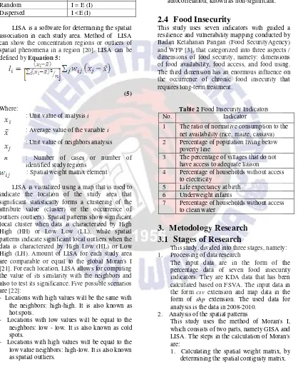
LISA is a software for determining the spatial association in each study area. Method of LISA can show the concentration regions or outliers of spatial phenomena in a region [20]. LISA can be defined by Equation 5:
(5) Where:
: Unit value of analysis i : Average value of the variable i : Unit value of neighbors analysis n : Number of cases or number of
identified study regions : Spatial weight matrix element
LISA is visualized using a map that is used to indicate the location of the study area that significant statistically forms a clustering of the attribute value (cluster) or the occurrence of outliers (outliers). Spatial patterns show significant local cluster when data is characterized by High High (HH) or Low Low (LL), while spatial patterns indicate significant local outliers when the data is characterized by High Low (HL) or Low High (LH). Amount of LISA for each study area are comparable or equal to the global Moran's I [21]. For each location, LISA allows for computing the value of its similarity with the neighbors and also to test its significance. Five possible scenarios are [22]:
- Locations with high values will be the same with the neighbors: high-high. It is also known as hot spots.
- Locations with low values will be equal to the neighbors: low - low. It is also known as cold spots.
- Locations with high values will be equal to the low value neighbors: high-low. It is also known as spatial outliers.
- Locations with low values will be equal to the low value neighbors: low-high. It is also known as spatial outliers.
- Locations that do not have spatial autocorrelation, known as non-significant.
2.4
Food Insecurity
This study uses seven indicators with guided a resilience and vulnerability mapping conducted by Badan Ketahanan Pangan (Food SecurityAgency) and WFP [3], that categorized into three aspects / dimensions of food security, namely: dimensions of food availability, food access, and food using. The third dimension has an enormous influence on the occurrence of chronic food insecurity that requires long-term treatment.
Table 2 Food Insecurity Indicators
No. Indicator
1 The ratio of normative consumption to the net availability (rice, maize, cassava) 2 Percentage of population living below
poverty line
3 The percentage of villages that do not have access to adequate liaison 4 Percentage of households without access
to electricity
5 Life expectancy at birth 6 Underweight infants
7 Percentage of households without access to clean water
3.
Metodology Research
3.1
Stages of Research
This study, divided into three stages, namely: 1. Processing of data research
The input data are in the form of the percentage data of seven food insecurity indicators. They are KDA data that has been calculated based on FSVA. The input data in the form csv extension and map data in the form of shp extension. The used data for analysis is the data in 2008-2010.
2. Analysis of the spatial patterns
This study uses the method of Moran's I, which consists of two parts, namely GISA and LISA. The steps in the calculation of Moran's are:
2. Calculating GISA, and the value of E (I). GISA is used to determine the correlation (cluster, random, dispersed) of an indicator in the entire observed region. 3. Calculating LISA. LISA is used to
determine the spatial pattern (hotspot, coldspot, outliers) on each visualized district visualized in the form of a map. The map illustrates regions of food insecurity in 2008-2010.
3. Analysis of study results
The results of this study are in the form of geographical information about food insecurity regions, which consists of the LISA maps and choropleth maps. Choropleth map is the out layer result of the map LISA in every year, which describes the food insecurity region in Boyolali Regency.
3.2 Desain and Architecture
Model
Figure 3 shows the design and architect model research. In general, the architect model can be seen in these 3 parts, they are:
1. The data is in .csv, they are : (1) RKN data from 2008 – 2010; (2) Percentage data of underprivileged community from 2008 – 2010; (3) Village percentage which does not has connection access 2008 – 2010; (4) Household percentage, which does not have electricity access from 2008 – 2010; (5) Life expectancy number 2008 – 2010; (6) Under standard weight of toddlers from 2008 – 2010; (7) Clean Water access percentage from 2008 – 2010.
2. Spatial analysis process like neighbors analysis, GISA and LISA
3. Visualization is used to visualized the research output like choropleth and LISA map
Figure 3. Desain and Architecture Model
4.
RESULT
The purpose of this study is to identify food insecurity regions in Boyolali Regency and find out how the correlation of the seven indicators among sub districts. The first stage to do is to calculate the percentage of each indicator according FSVA
Data
Data input
.csv
Data map
.shp
Process
Neighbor Analysis
LISA
GISA
Visualitation
Map of Food Insecurity
Area
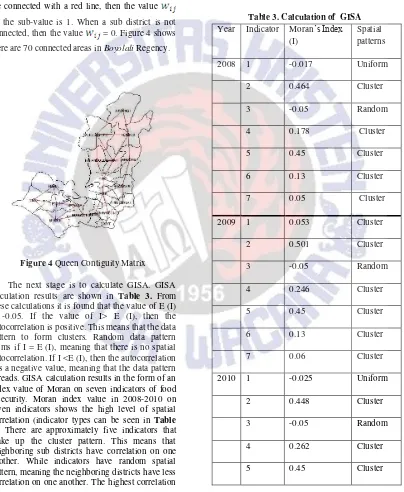
guidelines. Then calculate the spatial contiguity matrix, of which in this study uses queen contiguity matrix: the calculation of neighbor matrix by dividing any part of the common boundary region. Figure 4 shows the queen contiguity matrix in Boyolali Regency. Dot represents a sub district, and the red line shows the region of the neighboring districts. If sub districts are connected with a red line, then the value on the sub-value is 1. When a sub district is not connected, then the value = 0. Figure 4 shows there are 70 connected areas in Boyolali Regency.
Figure 4 Queen Contiguity Matrix The next stage is to calculate GISA. GISA calculation results are shown in Table 3. From these calculations it is found that the value of E (I) is -0.05. If the value of I> E (I), then the autocorrelation is positive. This means that the data pattern to form clusters. Random data pattern forms if I = E (I), meaning that there is no spatial autocorrelation. If I <E (I), then the autocorrelation has a negative value, meaning that the data pattern spreads. GISA calculation results in the form of an index value of Moran on seven indicators of food insecurity. Moran index value in 2008-2010 on seven indicators shows the high level of spatial correlation (indicator types can be seen in Table 2). There are approximately five indicators that make up the cluster pattern. This means that neighboring sub districts have correlation on one another. While indicators have random spatial pattern, meaning the neighboring districts have less correlation on one another. The highest correlation
between regions (close +1) is owned by the indicator percentage of population living below poverty line, with Moran index of 0.464. This index has potential to have converging spatial patterns (clusters). It means that percentage of population living below poverty line in neighboring sub districts in Boyolali Regency still have mutual correlation on each other.
Table 3. Calculation of GISA Year Indicator Moran’s Index
(I)
Spatial patterns
2008 1 -0.017 Uniform
2 0.464 Cluster
3 -0.05 Random
4 0.178 Cluster
5 0.45 Cluster
6 0.13 Cluster
7 0.05 Cluster
2009 1 0.053 Cluster
2 0.501 Cluster
3 -0.05 Random
4 0.246 Cluster
5 0.45 Cluster
6 0.13 Cluster
7 0.06 Cluster
2010 1 -0.025 Uniform
2 0.448 Cluster
3 -0.05 Random
4 0.262 Cluster
6 0.13 Cluster
7 0.03 Cluster
Figure 5 is a LISA map of underprivileged population in 2008. From Figure 5, shows that there are patterns of spatial clusters (clustered and correlated) in sub district Wonosegoro and Kemusu. These sub districts are marked with red color, which is a hotspot area (High-High). It means that these two sub districts have a high percentage of underprivileged population, and surrounded by sub districts that have a high percentage of underprivileged populations as well. Sub district that categorized as hotspot is a sub district that has potentially in food insecurity. Thus, such sub districts can be the focus in government's efforts to improve the welfare of the population. In addition, there is a district that has a High-Low value, the district Juwangi (marked in green). It shows that the percentage of the underprivileged population in Juwangi sub district is high, while the percentage in the surrounding regions are low. However, this condition does not affect the surrounding districts.
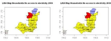
Figure 5 underprivileged population in 2008 In 2009-2010, there was a change in the spatial pattern of sub district Wonosegoro and Sambi. Wonosegoro sub district as hotspot region has become a non-significant region (Figure 6). It means that this sub district does not have a spatial correlation with the surrounding districts. A region can be a non-significant because there are factors limiting the distribution of the population from one region to the other regions, such as lakes, damaged roads, and other physical factors [Prasetyo, 2011]. On the contrary, in Sambi sub district, there are
significant spatial pattern changes from non-significant region to hotspot region. This means the percentage of the underprivileged population of Sambi sub district is quite high, at the surrounding sub districts with high percentage of underprivileged population as well.
Figure 6 underprivileged population in 2009-2010 Figure7 shows that in 2008, there are spatial pattern of local cluster in Juwangi, Wonosegoro and Boyolali sub districts. Hotspot regions that marked in red is Wonosegoro sub district. It is has potentially in food insecurity regions because it has high percentage of households without access to electricity and surrounded by the region with high percentage of households without access to electricity as well. Meanwhile, Juwangi and Boyolali sub districts included in the coldspot (Low-Low). It means that households residing in these two sub districts and the surrounding area have access to electricity.
Figure 7 households without access to electricity 2008
Figure 8 households without access to electricity 2009-2010
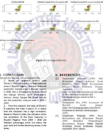
Figure 10 shows a map of LISA with seven indicators of food insecurity in 2008. Food insecurity area is area that included in the hotspot region in all indicators of food insecurity. From the figure shows that no region is experienced food insecurity. However, some districts has potentially affected by food insecurity because of the districts
included in the hotspot regions. There are hotspot regions on three indicators of food insecurity, which is on the indicator of percentage underprivileged population, the percentage of households without access to electricity. This means that these three indicators has correlation the occurrence of food insecurity in Boyolali Regency in 2008. On the indicator of underprivileged population percentage, there are two sub districts that included in hotspot region and have potential become food insecurity region i.e. namely Wonosegoro, and Kemusu sub districts. Wonosegoro district is also included in the hotspot region on indicator of household percentage without access to electricity.
Figure 10 LISA map 2008 In 2009, there has been a hotspot change
region with three same indicators as in 2008 (Figure 12). Changes occurred in the hotspot region on the percentage indicator of underprivileged population in two districts, namely Wonosegoro and Sambi sub districts. Wonosegoro sub district that originally was a hotspot area turned into non-significant regions. Meanwhile, the Sambi sub district that was as non-significant region turned into hotspot region.
In 2010, there were no changes in the spatial patterns of both the indicator and the region. Figure 12 shows a map of food insecurity regions
district, the high percentage of the underprivileged population causes this sub district experienced
potentially food insecurity.
Figure 12 LISA map 2009-2010
5.
CONCLUSION
Through this research, we can conclude that:
1. Based on neighbors analysis used
Mora ’s I Method, there is no food insecurity
areas in Boyolali Regency. However, there are
potentially insecure areas in Boyolali regency
in 2008, that is Wonosegoro, Kemusu, Ampel
dan Cepogo districts, while Wonosegoro,
Kemusu, Ampel, Cepogo dan Sambi districts
are the potentially insecure area in 2009 –
2010.
2. Fro this research, the i dex of Mora ’s 9 indicators the index is about +1, it means that the indicators has a high correlation.
Based o Mora ’s I dex, the i dicators which
has correlation of the food insecurity in
Boyolali Regency from 2008 – 2010 are Habitant percentage which live below the poor level and limited electricity access in the areas.
6.
REFERENCES
[1]
Departemen Pertanian, 2009, Peta Kerawanan Pangan Indonesia (Food Insecurity Atlas), Pusat Kewaspadaan pangan, Badan Ketahanan Pangan,September 2005,
(http://www.foodsecurityatlas.org/idn/count
ry/fsva-2009-peta-ketahanan-dan- kerentanan-pangan-indonesia/bab-1-pendahuluan).
[2] Karanganyar Pos, 2009, kecamatan di Boyolali rawan pangan, (http://www.karanganyarpos.com/2009/5- kecamatan-di-Boyolali-rawan-pangan-2435).
[4] Departemen Pertanian, 2010, Pusat Ketersediaan dan Kerawanan Pangan 2010, Kebijakan Pengembangan Ketersediaan Pangan. Bahan Paparan Workshop Dewan Ketahanan Pangan, 20-22 September 2010. Jakarta.
[5] Prasetyo, S. Y, 2010, Endemic Outbreaks of Brown Planthopper in Indonesia Using Exploratory Spatial Data Analysis. International Journal of Computer Science Issues, Vol. 9, Issue 5, No 1, September 2012.
[6] Tsai PJ, 2012, Application Of Moran's Test With An Empirical Bayesian Rate To Leading Health Care Problems In Taiwan In A 7-Year Period (2002-2008). Glob J Health Sci, 4 Juli 21012, 4(5):63-77. [7] Anselin, 1998, GIS Reseach Infrastructure
for Spatial Analysis of Real Estate Markets, Journal of Housing Research, Volume 9, Issue 1.
[8] Chen Y., 2010, On The Four Types of Weight Functions for Spatial Contiguity Matrix, Department of Geography, College of Environmental Sciences, Peking University, Beijing.
[9] LeSage, J. P., 1999, The Theory and Practice of Sapcial Econometrics, Department of Economics, University of Toledo.
[10] Vitton, P., 2010, Notes on Spatial Econometric Models, City and Regional Planning.
[11] Arrowiyah, Sutikno, 2009, Spatial Pattern Analysis Kejadian Penyakit Demam Berdarah Dengue Informasi Early Warning Bencana di Kota Surabaya, Institut Teknologi Surabaya.
[12] Harvey dkk, 2008, The North American Animal Disease Spread Model: A simulation model to assist decision making in evaluating animal disease incursions, Preventive Veterinary Medicine, Vol 82, Halaman 176-197.
[13] Dormann C. F., McPherson J.M., Methods to Account for Spatial Autocorrelation in
the Analysis of Species Distributional Data : a review, Ecography 30 : 609628, 2007, doi: 10.1111/j.2007.0906-7590.05171.x [14] Puspitawati Dewi, 2012. Pemodelan Pola
Spasial Demam Berdarah Dengue di Kabupaten Semarang Menggunakan Fungsi Moran’s I. Fakultas Teknologi Informasi, Universitas Kristen Satya Wacana.
[15] Celebioglu dan Dall’erba, 2008, Spatial Disparities across The Regions of Turkey : on exploratory spatial data analysis, Ann Reg Sci (2010) 45: 379-400, DOI 10.1007/s00168-009-0313-8.
[16] Anselin, L., 1995, Local Indicators of Spatial Association-LISA, Geographical Analysis, Vol. 27, No. 2 (April 1995) @ Ohio State University Press.
[17] Oliveau, S., Guilmoto, C. Z., 2010, Spatial Correlation And Demography. Exploring India’s Demographic Patterns, "XXVC Congrès International De La Population, Tours : France (2005)".
[18] BPS, Kecamatan dalam Angka 2010 , KabupatenBoyolali.
[19] Wonogiri pos, 2013,
http://www.wonogiripos.com/2013/soloray
a/Boyolali
/duh-desa-ngendroloka-belum-tersentuh-listrik-381716
[20] Celebioglu dan Dall’erba, 2008, Spatial Disparities across The Regions of Turkey : on exploratory spatial data analysis, Ann Reg Sci (2010) 45: 379-400, DOI 10.1007/s00168-009-0313-8.
[21] Anselin, L., 1995, Local Indicators of Spatial Association-LISA, Geographical Analysis, Vol. 27, No. 2 (April 1995) @ Ohio State University Press.