arXiv:1709.04387v1 [q-fin.MF] 13 Sep 2017
Welfare effects of information and rationality in
portfolio decisions under parameter uncertainty
Michele Longo
∗Alessandra Mainini
†September 14, 2017
Abstract
We analyze and quantify, in a financial market with parameter uncer-tainty and for a Constant Relative Risk Aversion investor, the utility effects of two different boundedly rational (i.e., sub-optimal) investment strategies (namely, myopic and unconditional strategies) and compare them between each other and with the utility effect of full information. We show that ef-fects are mainly caused by full information and predictability, being the effect of learning marginal. We also investigate the saver’s decision of whether to manage her/his portfolio personally (DIY investor) or hire, against the pay-ment of a managepay-ment fee, a professional investor and find that delegation is mainly motivated by the belief that professional advisors are, depending on investment horizon and risk aversion, either better informed (“insiders”) or more capable of gathering and processing information rather than their ability of learning from financial data. In particular, for very short investment hori-zons, delegation is primarily, if not exclusively, motivated by the beliefs that professional investors are better informed.
Keywords: Portfolio choice; Parameter uncertainty; Return predictability; Bayesian learning; Bounded rationality; DIY investor. JEL Classification: G11, G14.
∗Universit`a Cattolica del Sacro Cuore, Largo Gemelli, 1, Milano, 20123, Italy. E-mail address:
†Universit`a Cattolica del Sacro Cuore, Largo Gemelli, 1, Milano, 20123, Italy. E-mail address:
1
Introduction
Traditional portfolio management models assumed, among others, complete observ-ability of markets’ parameters and fully rational agents. But, as soon as empirical tests revealed limits of these models to explain financial data, a vast literature has grown with the aim of relaxing some of the classical assumptions. We refer to Pastor and Veronesi [19] for a review of recent work on parameter uncertainty and learning in finance; whereas, reasons for incorporating bounded rationality in financial models can be found in the surveys on behavioral finance by De Bondt and Thaler [10] and Barberis and Thaler [1].
In this paper we analyze and quantify the welfare effects – in terms of additional fraction of initial wealth that makes two investment strategies indifferent – of two boundedly rational investment behaviors in a continuous-time financial market with parameter uncertainty,1 and compare them between each other and with the effect of uncertainty measured by the additional fraction of initial wealth that makes a rational agent indifferent between a full information and a partial information sce-nario. In particular, we consider expected utility investors with Constant Relative Risk Aversion (CRRA) preferences over terminal wealth that trade in a continuous-time financial market with a risk-less bond and a risky asset, where the market price of risk is represented by a – possibly unobservable – random variable with Gaussian prior distribution.2 In a dynamic context, parameter uncertainty has two effects. The first is the predictive role of observable quantities (in our setting the observable market price of risk tells about the distribution of the unobservable variable). The second effect has to do with the fact that uncertainty changes over time. Indeed, as new information comes to light through further observation, the investor updates its posterior distribution for the unobserved parameter, thus changing the investment opportunity set which, in turn, produces an hedging demand due to the possibility of learning from these changes. In this setting, agents may be boundedly rational in that they either do not behave dynamically (i.e., they do not learn from fluctuations in the conditional distribution of the unobserved parameter) but process information properly, we refer to them asmyopic investors,3 or they also lack of competence in
1
In this paper, the expressions “parameter uncertainty”, “partial observation”, and “partial information” are used interchangeably.
2
Since we are interested in valuing and comparing conditions such as better access to informa-tion, or better ability to process it or to behave dynamically, we abstract from transaction costs and others types of market frictions such as limited trading and assume that investors trade continuously at zero costs.
3
Myopic strategies have also been proved to be optimal in certain optimization-based portfolio
gathering and processing information (i.e., they completely disregard available in-formation provided by prices, thus ignoring predictability of assets returns), we call themunconditional investors.4 Our explicit results allow us to decompose the utility effect in passing from a partially informed unconditional investor (the least informed and “able”) to a fully informed rational investor (the best informed and “able”) into the sum of the effects of predictability, learning, and full information. This decomposition, apparently new in this context, enables to show that welfare effects of parameter uncertainty are mainly caused, depending on risk aversion and invest-ment horizon, by full information and/or predictability, being the effect of learning marginal. In particular, in the short run, effects are almost exclusively associated to full information and then to predictability and learning, with the value of the latter negligible compared with the previous two.
Then, the analysis is adapted to investigate the saver’s choice of whether to man-age her/his portfolio personally (DIY investor) or hire, at some cost, a professional investor. Our findings support the idea that delegation is mainly motivated by the beliefs that professional investors are either better informed (“insiders”) or more ca-pable of gathering and processing information rather than their ability of learning from financial data. In particular, for very short investment horizons, delegation is primarily, if not exclusively, motivated by the beliefs that professional investors are better informed. Moreover, it is also suggested that investors with a coefficient of relative risk aversion between 0 and 1 are presumably the more interested in delega-tion.
Our work is related to the literature on continuous-time financial models with parameter uncertainty. We cite, among others, Brennan [5], Lakner [16], Karatzas and Zhao [14], Rogers [23], Xia [24], Honda [12], Rieder and B¨auerle [21], Cvitani´c et al. [9], Bj¨ork et al. [2], Longo and Mainini [18]. However, almost all these papers are mainly concerned with portfolio allocation effects of either bounded rationality or full information rather than with the effects on agents’ utility and the few of them that consider the latter effects confine their analysis either to special cases in terms of agent’s risk aversion or to a single type of sub-optimal strategy (see, for instance, Browne and Whitt [8], Brennan and Xia [7], Cvitani´c et al. [9]) or just to uncertainty (see, for example, Karatzas and Zhao [14], Brendle [4]). Branger et al. [3] analyze,
are not concerned with the issue of rationalizing certain, apparently boundedly rational, behaviors but rather to evaluate and compare them.
4
We focus on these sub-optimal behaviors because, by citing De Bondt and Thaler [10] (pp. 385-386), it is not realistic to assume that everyone in the economy is “as smart as Sandy Grossman”, neither plausible that “everyone looks toward the future in a way that would make econometricians
in a more general setting, portfolio and welfare effects of learning and ambiguity in a fashion similar to the one employed in the present work.
Although the way of behaving rationally is often unique within a certain paradigm, there are several ways of being boundedly rational: potentially, any sub-optimal strategy may represent a boundedly rational behavior within the model it belongs to. In this paper we consider two types of sub-optimal policies, that is myopic
and unconditional, but other types of sub-optimal behaviors have been explored in continuous-time portfolio management models. For instance, sub-optimal leverage or sub-optimal diversification have been considered by Brennan and Torous [6], where, in a complete information setting, the Authors show that the cost of departing from the optimal allocation to the risky asset (sub-optimal leverage), even of a factor as high as.5, is modest (and, by order of magnitude, comparable with reasonable port-folio management fees), whereas the cost of poor diversification (i.e., portfolios where some assets are omitted) may be much higher. Larsen and Munk [17] confirm, in a more general setting, the conclusions of Brennan and Torous [6] about the welfare loss of poor diversification. They also analyze near-optimal strategies (i.e., strate-gies obtained by small perturbations from the optimal portfolio weights) and myopic strategies, finding that losses associated to the latter investment policies are limited. Rogers [23] analyzes the sub-optimal strategy named relaxed: that is, the investor changes portfolio allocations at fixed times (the extreme case being thebuy-and-hold
strategy). The Author provides, in a completely observable model, a power expan-sion of the corresponding cost and shows that it is not so high, at least if compared with the cost of uncertainty. In Haugh et al. [11], the Authors develop an algorithm to evaluate sub-optimal policies in portfolio problems with trading constraints by means of bounds on the utility loss associated to a given sub-optimal strategy and apply the algorithm to evaluate the quality of unconditional (that they call static) and myopic strategies in the context of return predictability.
management to a professional investor. Section 5 concludes.
2
The investment problem
In a continuous-time frictionless financial market, an investor with investment hori-zon T > 0 and initial wealth x > 0 trades two assets: a risk-free asset (bond) with constant interest rate r ≥ 0 and a risky asset (stock) whose price process (St)t≥0 satisfies the equation
dSt =St((r+σΘ)dt+σdWt), (2.1)
where (Wt)t≥0 is a standard Brownian motion, σ is a positive constant, and Θ, the
market price of risk, is a random variable independent of (Wt)t≥0 and with known prior distribution normally distributed with meanθ0 and variancev0. If the investor chooses the trading strategy π= (π(t))t∈[0,T], where π(t)∈Rrepresents the fraction of wealth invested in the risky asset at time t, then his/her wealth (Xt)t≥0 evolves
according to the budget equation
dXt=rXtdt+σπ(t)Xt(Θdt+dWt), X0 =x, (2.2)
and we assume that he/she enjoys expected utility (from terminal wealth)
E[uγ(XT)], (2.3)
where
uγ(x) :=
x1−γ
1−γ, γ >0, γ 6= 1,
lnx, γ = 1,
(2.4)
being γ the investor’s coefficient of relative risk aversion. Investors with γ > 1 are known in literature as conservative, whereas those with risk aversion 0 < γ < 1 are called aggressive.5 In order to avoid infinite expected utility, we assume throughout the paper that parameters satisfy the condition γ(1 +v0T)−v0T > 0. Notice that: (i) if we fix v0 > 0 and γ > 0, then, if γ ≥ 1, T can range in the entire positive half-line, whereas, if 0 < γ <1, the condition holds for T <T¯ :=γ/(v0(1−γ)); if we fix v0 >0 and T ≥ 0, then we consider all γ > γ¯ :=v0T /(1 +v0T) (notice that 0<γ <¯ 1).
We now determine explicitly the expected utility in (2.3) under several specifica-tions about agents’ knowledge of Θ and/or agents’ rationality. In particular, we first
5
assume that the investor knows the true distribution of Θ and invests accordingly (Section 2.1). Then, we consider a setting where the investor does not observe Θ but knows only its prior, and calculate the expected utilities of a rational (i.e., an investor that, by observing stock returns, continuously updates her/his beliefs about the unobserved market price of risk, Section 2.2.1), a myopic (i.e., an investor that properly learns about the unobservable market price of risk by observing stock re-turns, but ignores the dynamic aspect of the investment decision, Section 2.2.2) and an unconditional (i.e., an investor that completely disregards available information provided by the observed market price of risk and sticks to its prior, Section 2.2.3) agent.
2.1
Fully informed investors
A fully informed and rational investor (I) observes Θ as well as (Wt)t≥0 and maxi-mizes the expected value (2.3), subject to the wealth dynamics (2.2), over all (FtΘ,W
)-progressively measurable (and integrable) investment strategiesπ, where (FtΘ,W)t≥0 is the filtration generated by Θ and (Wt)t≥0. The agent invests according to the
standard Merton’s strategy
πγI(t) = Θ
σγ, 0≤t≤T, γ >0, (2.5)
and enjoys the expected utility (see Appendix 6.1)
VI(x;γ, T) =
x1−γ
1−γ exp ϕ
I(γ, T)θ2
0+ψI(γ, T)
, γ >0, γ 6= 1,
lnx+rT + θ 2 0T
2 +
v0T
2 , γ = 1,
(2.6)
where, forT ≥0,γ >0 and γ 6= 1,
ϕI(γ, T) := (1−γ)T 2(γ(1 +v0T)−v0T)
(2.7)
and
ψI(γ, T) := 1 2ln
γ
γ(1 +v0T)−v0T
+r(1−γ)T. (2.8)
2.2
Partially informed investors
resulting portfolio problem, which is ofpartial informationtype, has been extensively studied in literature (see, among others, Karatzas and Zhao [14], Rogers [23], Rieder and B¨auerle [21], Bj¨ork et al. [2], and Pham [20]). Typically, the problem is first reduced, by means of filtering techniques, within a complete observation setting and then solved either by martingale methods or by dynamic programming techniques. Since the analysis of such problems is by now standard, we just recall the definitions we will use later to represent different investment strategies and refer to the literature for details (see, for instance, Rishel [22], Karatzas and Zhao [14], or Rogers [23], Section 6). Let FS
t
t≥0 be the filtration generated by (St)t≥0 and define the process
dYt= ˆΘ(t, Yt)dt+dWˆt, Y0 = 0, (2.9)
where
ˆ
Θ(t, y) := θ0+v0y 1 +v0t
(2.10)
and ( ˆWt)t≥0 is a Brownian motion w.r.t. the observable filtration FtS
t≥0. Then
ˆ
Θ(t, Yt) =E[Θ| FtS], 0≤t≤T, (2.11)
(i.e., ˆΘ(t, Yt) is the time t Bayesian estimation of Θ, conditional on the available
information FS t ) and
dXt =rXtdt+σπ(t)Xt( ˆΘ(t, Yt)dt+dWˆt), X0 =x, (2.12)
represents the investor’s budget constraint in terms of observable quantities, where
π is a FS t
-progressively measurable (and integrable) investment strategy.
2.2.1 Rational investors
In a dynamic context under partial information, a rational investor (R) properly updates his/her beliefs about the unobservable parameter Θ, conditional on the observed market price of risk, and hedges against future changes in the investment opportunity set, when building his/her portfolio, by learning from fluctuations in the filtered marked price of risk. Formally, such an investor maximizes (2.3) over all FS
t
-progressively measurable (and integrable) investment strategies π, under the two-dimensional state dynamics (2.9), (2.12). This is acomplete observation and Markovian control problem that is solved by using dynamic programming techniques (see Appendix 6.2). The optimal investment strategy and the expected utility are, respectively,
πRγ(t) = Θ(ˆ t, Yt)
σγ +
ˆ Θ(t, Yt)
σγ
(1−γ)(T −t)v0
γ(1 +v0T)−v0T +v0t
and
Amyopic investor (M) properly updates, by means of the Bayesian estimator (2.11), the conditional distribution of Θ but ignores the hedging demand associated to fluc-tuations on the filtered market price of risk (that is, he/she considers the estimation as it were constant from t onwards). Hence, he/she chooses the investment policy6
πMγ (t) = Θ(ˆ t, Yt)
σγ , 0≤t ≤T, γ >0, (2.17)
and enjoys an expected utilityVM, given by (2.3), where the wealth process evolves
according to (2.12) withπ =πM
γ . After some algebra (see Appendix 6.3) one obtains:
VM(x;γ, T) =
Notice that, according to Kuwana [15], the logarithmic investor is myopic, that is πM
1 (t) =
πR
ψM(γ, T) := 1 2
ln r2−r1
r2(1 +v0T)r2−r1 −r1
+r2ln(1 +v0T)
+r(1−γ)T, (2.20)
and r1, r2, withr1 < r2, are the solutions of the quadratic equation:
r2+
2
γ −1
r+ 1−γ
γ = 0. (2.21)
2.2.3 Unconditional investors
Here the degree of bounded rationality is even more severe in that anunconditional investor (U) do not even update the conditional distribution of Θ and considers the market price of risk constant and equal to its unconditional mean θ0 =E[Θ] for the entire investment period, thus ignoring both predictability of and learning from the available information provided by stock returns. Notice that unconditional investors are also myopic because there is no possibility of learning since the investment op-portunity set is constant. The unconditional strategy takes the form (cf. Haugh et al. [11] or Brennan and Xia [7])
πUγ(t) = θ0
σγ, 0≤t ≤T, γ >0, (2.22)
and the corresponding expected utility,VU, is given by (2.3), whereX
T is determined
via the wealth dynamics (2.12) withπ=πU
γ. After some algebra (see Appendix 6.4),
we get:
VU(x;γ, T) =
x1−γ
1−γ exp ϕ
U(γ, T)θ2
0+ψU(γ, T)
, γ >0, γ 6= 1,
lnx+rT +θ 2 0T
2 , γ = 1,
(2.23)
where, forT ≥0,γ >0 and γ 6= 1,
ϕU(γ, T) := (1−γ)(γT + (1−γ)v0T 2)
2γ2 (2.24)
and
3
Value of full information, predictability and
learn-ing
We compare the scenarios studied in the previous sections and quantify the difference between any two of them in terms of additional fraction of initial wealth needed to obtain the same expected utility.7 By observing that, for all x > 0, γ > 0 and
T >0,8
VU(x;γ, T)≤VM(x;γ, T)≤VR(x;γ, T)≤VI(x;γ, T), (3.1)
we introduce on the set{I, R, M, U}, where I, R, M and U refer, respectively, to the scenarios analyzed in Sections 2.1, 2.2.1, 2.2.2 and 2.2.3, the order relationU -M
-R - I, and, for i, j ∈ {I, R, M, U}, with i - j, we define Cij as the quantity such
that
Vi(x;γ, T) =Vj(x(1−Cij);γ, T). (3.2)
Since the passage from scenarioi to scenario j, with i-j, is valuable and, possibly, onerous,Cij may be seen as the maximum cost,9 in terms of fraction of initial wealth, that an investor acting in scenario i is willing to pay to move to scenarioj (a reser-vation price). In particular, in a dynamic context with parameter uncertainty, CU M
may be considered a measure (in terms of additional fraction of initial wealth) of the value of the sole predictability (i.e., the value of using the conditional distribution for the unobserved market price of risk), CM R a measure of the value of learning
(i.e., the value of behaving dynamically), once predictability has been considered,
CRI a measure of the value of full information once rationality (i.e., predictability
and learning) has been considered, and CU I a measure of the benefit of considering the three aspects of portfolio decision all together. Notice that Cij represents the
cost over the entire investment horizon – a sort of cumulated or compound cost –, in Section 4 we introduce an annual version of the cost.
Thanks to the explicit form of expected utilities VI, VR, VM and VU, we have:
Cij =Cij(γ, T) = 1−exp
ϕi(γ, T)−ϕj(γ, T)
1−γ θ
2 0 +
ψi(γ, T)−ψj(γ, T)
1−γ
, (3.3)
7
A similar analysis, though with a different cost definition, and just for the logarithmic utility and without considering the myopic strategy, is performed in Browne and Whitt [8].
8
Moreover, for eachi, the expected utility of the logarithmic investorVi(x; 1, T) is the limit of
Vi(x;γ, T)−1/(1−γ), asγ→1, for anyx, T >0.
9
Our definition of cost is identical to the notion of utility loss defined in Branger et al [3]. It
is also similar to the concept of wealth-equivalent utility loss employed in Larsen and Munk [17].
Moreover, 1−Cij is called efficiency in Rogers [23] and its inverse is the ratio of the certainty
i, j ∈ {I, R, M, U}, γ > 0, γ 6= 1. Costs are independent of the initial wealth x and logarithmic costs (i.e.,γ = 1), which have the following simple form:
CU M(1, T) = 1−e−v0T /2
(1 +v0T)1/2, (3.4)
CM R(1, T) = 0, (3.5)
CRI(1, T) = 1−(1 +v0T)−1/2, (3.6)
are equal to the limits, asγ →1, of the corresponding power costs. Representation (3.3) allows to write the identity
CU I = 1− 1−CU M
1−CM R
1−CRI
, (3.7)
which implies, at least when costs are sufficiently low – and this is true for significant ranges of parameters γ and T, and for reasonable values of the other parameters –, the following approximation:
CU I ≈CU M +CM R+CRI. (3.8)
That is, the cost in passing from a partially informed unconditional investor (the least informed and “able”) to a fully informed rational investor (the best informed and “able”) is split into the sum of the costs of predictability, learning, and full information. Notice that (3.7) and (3.8) hold true also for the logarithmic case (i.e.,
γ = 1).
The rest of the section is devoted to the analysis of CU M, CM R, CRI and the
goodness of approximation (3.8) with respect to the investment horizon T and the risk aversionγ. We start from the investment horizon. Standard calculus yields:10
CU M(γ, T) = v 2 0 4γT
2+o T2
, T →0, (3.9)
CM R(γ, T) =o T2
, T →0, (3.10)
CRI(γ, T) = v0 2γT +
v2 0 4γ
1 2γ −2
T2+o T2
, T →0, (3.11)
CU I(γ, T) = v0 2γT +
v2 0 4γ
1 2γ −1
T2+o T2
, T →0, (3.12)
for each γ >0. Hence, all costs vanish as T shrinks to 0 and, by observing that
CU I(γ, T) =CU M(γ, T) +CM R(γ, T) +CRI(γ, T) +E(γ, T), (3.13)
10
where the error E(γ, T) is such that
E(γ, T) = o T2
, T →0, (3.14)
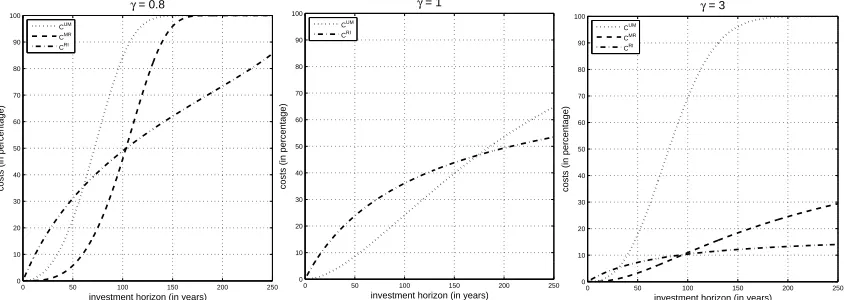
we expect approximation (3.8) to be extremely accurate for sufficiently short invest-ment horizons, as simulations ahead in the section confirm. We also notice that, in the short run, costs are mainly motivated by full information and then by predictabil-ity and learning, with the value of the latter negligible compared with the previous two. Reasonably, predictability and learning display their effects in the long run. Costs’ behavior as the investment horizon gets longer depends onγ. We distinguish three cases: (i) γ >1, costs exist for all T ≥0 and
lim
T→∞ C
U M(γ, T) = lim
T→∞ C
M R(γ, T) = 1, lim
T→∞ C
RI(γ, T) = 1−p
1−1/γ; (3.15)
(ii)γ = 1 (the logarithmic case, see (3.4)-(3.6)), costs exist for allT ≥0,CM R(1, T) =
0, for allT, and
lim
T→∞ C
U M(1, T) = lim
T→∞ C
RI(1, T) = 1; (3.16)
(iii) 0< γ < 1, costs exist for allT not exceeding ¯T, and
lim
T→T¯ C
U M(γ, T) = CU M γ,T¯
<1, lim
T→T¯ C
M R(γ, T) = lim T→T¯ C
RI(γ, T) = 1.
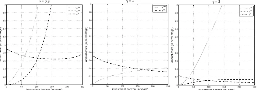
(3.17) Notice that for very long investment horizons – though financially implausible – costs, exceptCM R(1, T), which is identically 0, become relevant (see Figure 2) and,
as a consequence, approximation (3.8) does not hold. Nevertheless, for financially reasonable values of the parameters, our simulations show that the approximation applies well for realistic investment horizons such as those not exceeding 30 years (see Table 1). Lastly, since costs refer to the entire investment horizonT, we expect them to increase with respect toT and, indeed, it can be proved (though, with some algebra) that, for all γ > 1, CU M, CM R and CRI are increasing with respect to T.
CU M and CRI are increasing also for γ = 1 (see (3.4)-(3.6)).
We now turn to costs’ behavior with respect to the coefficient of relative risk aversion γ. We recall that, for any fixed T >0, costs exist for all γ >¯γ =v0T /(1 +
v0T). We have
lim
γ→∞ C
U M(γ, T) = lim
γ→∞ C
M R(γ, T) = lim
γ→∞ C
RI(γ, T) = 0, (3.18)
risk aversion increases because investment in the risky asset (see, expressions (2.5), (2.13), (2.17) and (2.22)), the only one that carries uncertainty, approach to 0 as
γ increases to infinity, hence, information affects a very little part of the investor’s wealth and, consequently, its value becomes negligible. As already noticed, costs tend to the logarithmic case as γ approaches to 1, and, as γ →¯γ, we have
lim
γ→¯γ C
U M(γ, T) =CU M(¯γ, T)<1, lim γ→¯γ C
M R(γ, T) = lim γ→¯γ C
RI(γ, T) = 1. (3.19)
Finally, CRI(γ, T) is decreasing with respect to γ for all T >0, whereas simulations
ahead show that other costs are not monotonic in general.
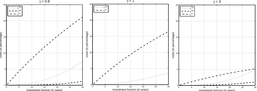
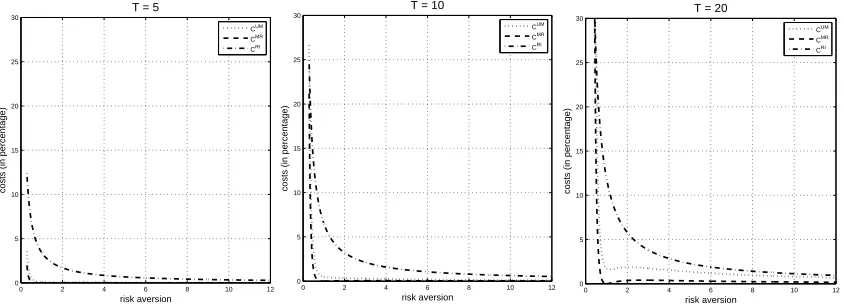
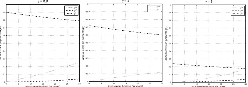
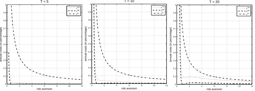
To gain insights about the importance of predictability, learning, and full infor-mation in portfolio management, we assume that time is measured in years and plot the above costs: (i) against investment horizonT, forγ = 0.8,1,3, in Figures 1 and 2, and (ii) against risk aversionγ, forT = 5,10,20, in Figure 3. In particular, for each value ofγ (in Figures 1 and 2) andT (in Figure 3), we provide two graphs, vertically aligned: the upper graph represents CU M,CM R and CRI; the lower graph shows the
relative contribution (in percentage) of each cost. We plot all costs for investment horizons T not exceeding 30 andγ ≤12, whereas, for the other parameters we use a specification estimated in Brennan [5]. In particular, the risk free rate is 5%, and the annual standard deviationσ of the risky asset on the market is 20.2% (see Brennan [5], Section 3, for a detailed explanation about the derivation of these values). On what concerns the prior of Θ, given a value for σ, we consider, again as in Brennan [5], Θ normally distributed with mean θ0 = 0.08/σ and variancev0 = (0.0243/σ)2.
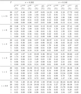
Table 1 reports the numerical values of the cost of predictability CU M, the cost
of learning CM R, the cost of full information CRI, the cost of the three previous
features all together CU I and the absolute value of the error E in decomposition
(3.13) (all expressed in %) for values of T and γ commonly used in literature for these simulations.11 The computations are performed, as in Brennan [5], for two specifications of the annual standard deviation of the risky asset on the market σ: that is, 20.2% and 14%. As for figures, Θ is normally distributed with mean 0.08/σ
and variance v0 = (0.0243/σ)2.12
The following observations are in order: (a) The upper graphs of Figures 1 and 2 show, consistent with the theory, that all costs increase in the investment horizon
T although with a lower intensity the higher the risk aversion. It is also evident (see
11
Cf. Brennan [5], Xia [24], Honda [12], Cvitani´c et al. [9], Larsen and Munk [17] and Longo and Mainini [18].
12
In Brennan [5] it is also considered Θ normally distributed with mean 0.08/σ and variance
v0= (0.0452/σ) 2
Figure 1: Cumulated costs against investment horizon T (≤ 30) for σ = 0.202,
investment horizon (in years)
costs (in percentage)
investment horizon (in years)
costs (in percentage)
investment horizon (in years)
costs (in percentage)
investment horizon (in years)
costs (in percentage)
investment horizon (in years)
costs (in percentage)
investment horizon (in years)
Figure 2: Cumulated costs against investment horizon T(≤ 250) for σ = 0.202,
investment horizon (in years)
costs (in percentage)
investment horizon (in years)
costs (in percentage)
investment horizon (in years)
costs (in percentage)
investment horizon (in years)
costs (in percentage)
investment horizon (in years)
costs (in percentage)
investment horizon (in years)
Table 1: Cumulated costs for θ0 = 0.08/σ and v0 = (0.0243/σ)2.
T σ= 0.202 σ= 0.140
CU M CM R CRI CU I |E| CU M CM R CRI CU I |E|
(%) (%) (%) (%) (%) (%) (%) (%) (%) (%)
γ= 11
30 2.17 0.46 1.39 3.97 0.05 14.23 1.93 2.18 17.72 0.62 20 0.74 0.18 1.03 1.93 0.02 5.15 0.91 1.72 7.63 0.15 10 0.12 0.03 0.58 0.72 0.01 0.82 0.20 1.06 2.06 0.02 5 0.02 0.00 0.31 0.33 0.00 0.13 0.03 0.60 0.76 0.00 1 0.00 0.00 0.06 0.07 0.01 0.00 0.00 0.13 0.14 0.01
γ= 6
30 3.46 0.74 2.56 6.63 0.13 21.83 3.23 4.04 27.41 1.69 20 1.19 0.28 1.89 3.33 0.03 8.11 1.50 3.18 12.37 0.42 10 0.20 0.05 1.06 1.30 0.01 1.32 0.31 1.95 3.55 0.03 5 0.04 0.01 0.56 0.61 0.00 0.22 0.05 1.10 1.36 0.01 1 0.00 0.00 0.12 0.12 0.00 0.00 0.00 0.24 0.25 0.01
γ= 4
30 4.41 0.96 3.86 8.97 0.26 26.97 4.31 6.12 34.40 3.00 20 1.53 0.36 2.85 4.68 0.06 10.22 1.96 4.82 16.22 0.78 10 0.26 0.06 1.59 1.91 0.00 1.70 0.40 2.94 4.97 0.07 5 0.05 0.01 0.85 0.90 0.01 0.29 0.07 1.65 2.00 0.01 1 0.00 0.00 0.18 0.18 0.00 0.01 0.00 0.37 0.37 0.01
γ= 3
30 4.93 1.07 5.18 10.82 0.36 29.54 5.03 8.25 38.60 4.22 20 1.74 0.40 3.81 5.86 0.09 11.32 2.23 6.48 18.92 1.11 10 0.31 0.06 2.13 2.49 0.01 1.93 0.44 3.94 6.20 0.11 5 0.06 0.01 1.13 1.20 0.00 0.34 0.07 2.21 2.61 0.01 1 0.00 0.00 0.24 0.24 0.00 0.01 0.00 0.49 0.50 0.00
γ= 1
30 3.61 0.00 16.50 19.51 0.60 12.19 0.00 27.53 36.36 3.36 20 1.75 0.00 11.94 13.47 0.22 6.34 0.00 21.01 26.01 1.34 10 0.48 0.00 6.53 6.98 0.03 1.88 0.00 12.34 13.98 0.24 5 0.12 0.00 3.43 3.55 0.00 0.51 0.00 6.78 7.26 0.03 1 0.01 0.00 0.72 0.72 0.01 0.02 0.00 1.47 1.50 0.01
γ= 0.8
also Table 1) that costs are moderate in the short run (T ≤ 5) and, according to the theoretical analysis, almost entirely attributable to full information. Interesting to notice is the relative contribution of each single cost. One can observe from the lower graphs of Figure 1 that, at least for reasonable investment horizons (T ≤30),13 the contribution of learning is the less valuable being, on average, less than 10% of the entire cost, whereas, the remaining 90% is divided, in proportions that depend on risk aversion and investment horizon, between predictability and full information. Moreover, the relative importance of predictability increases in the investment hori-zon for any givenγ, whereas the contribution of full information goes in the opposite direction. This is reasonable since the Bayesian estimator (2.11) converges to Θ ast
increases to infinity. In other words, as new information comes to light, the approx-imation of Θ gets better and, consequently, the additional value of full information diminishes.
(b) According to the previous analysis, the upper graphs of Figure 3 show that costs shrinks to 0 as risk aversion increases, though not all in a monotonic way. Furthermore, costs may be relevant for investors with risk aversion less than 1 also for relatively short investment horizons. For example (see Table 1), an investor with
γ = 0.8, an investment horizon of 20 years, and σ = 0.140 may value predictability 15.34%, learning 3.27%, and full information 27.20% of the initial wealth. Observe that when costs are relevant, such as in the previous specification, approximation (3.8) is less accurate, as the error may be as high as 20%. Moreover, the lower graphs of Figure 3 show that, for any givenT, the relative contribution of predictability and learning increase forγ >1 and decrease for γ <1, whereas the relative contribution of full information goes in the opposite direction, and this behavior is exacerbated for longer investment horizons. This means that the logarithmic investor (i.e.,γ = 1) not only gives zero value to learning (i.e.,CM R= 0), which is well known in literature (cf.
Kuwana [15]), but also assigns the lowest relative value to predictability (although this value increases in the investment horizon as the middle-lower graphs of Figures 1 and 2 show). In other words, the logarithmic investor gives, among CRRA investors, the lowest relative value to conditional information.
(c) As already noticed, the welfare effect of learning is the less valuable in the context of dynamic portfolio choice with parameter uncertainty. This is consistent with the findings of Haugh et al. [11] and Larsen and Munk [17]. However, Haugh et al. [11] analysis leaves room for the possibility that predictability may have relevant welfare effects and, indeed, for reasonable parameters’ values, our simulations show that this is the case for sufficiently long investment horizons. It is worth noticing
13
that, despite the fact that the cost of behaving myopically is not very relevant, the hedging demand, defined as the differenceπR
γ−πγM (see (2.13) and (2.17)), associated
to learning may be substantial as it is shown in Brennan [5] and, in a more general setting, in Longo and Mainini [18] (see also Haugh et al. [11]).
4
DIY
vs
Delegated portfolio management
In this section, we use the previous analysis to investigate the saver’s decision of whether to manage her/his portfolio personally, DIY investor, or hire, at some cost, a professional investor. We abstract from possible conflicts of interests arising from agency contracts by assuming that financial intermediaries may be compelled by authorities to act according to client’s risk profile and financial situation. 14 We consider the case where a saver of typei∈ {I, R, M, U}faces the possibility of dele-gating, against the payment of a fee, her/his portfolio management to a professional investor of typej ∈ {I, R, M, U}, with i-j. Since portfolios’ management fees are typically on annual basis and expressed as a percentage of the invested wealth, we measure time in years and assume that a saver of typei hires a professional investor of type j as long as the annual commission fee does not exceed the quantity cij,
which is the annual cost defined by the indifference relation:
Vi(x;γ, T) =Vj(x(1−cij)T;γ, T). (4.1)
That is,
cij =cij(γ, T) = 1−exp
ϕi(γ, T)−ϕj(γ, T)
(1−γ)T θ
2 0+
ψi(γ, T)−ψj(γ, T)
(1−γ)T
= 1−(1−Cij)1/T,
14
For example, within the European Economic Community, theMarkets in Financial Instruments
where Cij is the cumulated cost defined in (3.3). Notice that, costs are again
inde-pendent of the initial wealth x and logarithmic costs (i.e., γ = 1),
cU M(1, T) = 1−e−v0/2
(1 +v0T)1/(2T), (4.2)
cM R(1, T) = 0, (4.3)
cRI(1, T) = 1−(1 +v0T)−1/(2T), (4.4)
are equal to the limits, as γ →1, of the corresponding power costs. cij is an annual
version of the cost (3.3) (for an explanation of the definition, we refer the reader to Brennan and Torous [6], Section 2.3) and may be seen as the maximum annual management fee, in terms of fraction of initial wealth, that a saver of type i, risk aversion γ and investment horizon T, is prepared to pay for hiring a professional investor of type j, with i-j. Moreover, a decomposition similar to (3.8) holds also in this case, that is
cU I ≈cU M +cM R+cRI, (4.5)
and it can be used to assess the importance of predictability, learning and full in-formation in the saver decision of delegating the portfolio management: it tells us about the more valuable investment advisory services by a saver. In fact, cU M, cM R
andcRI may be considered the parts of a management fee attributable, respectively,
to advices about predictability, learning and full information.
Similarly to the previous section, we first analyse costs cU M, cM R, cRI and
ap-proximation (4.5) in generality with respect to risk aversion and investment horizon and then simulations analogous to those of the previous section will provide practical insights. Indeed, Table 2, whose description is similar to Table 1, reports the annual costs for the same parameter configuration of Table 1. Figures 4, 5 and 6 represent respectively the annual versions of Figures 1, 2 and 3.
We start from the investment horizon T. For each γ > 0, the following Taylor expansions hold in a (right) neighborhood of T = 0:
cU M(γ, T) = v
Hence, contrary to the cumulated case, not all costs vanish as T goes to 0: indeed,
lim
T→0 c
U M(γ, T) = lim T→0 c
but
lim
T→0 c
RI(γ, T) = 1−exp
−v0
2γ
>0. (4.11)
Consistent with the previous section, in the short run, also annual costs are mainly explained by full information, then by predictability and residually by learning. We can say even more, for very short investment horizons delegation is primarily, if not exclusively, motivated by the beliefs that professional investment advisers are better informed (“insiders”) rather than their ability of gathering and processing information or learning from financial data, and this is reasonable since within this time lag there is no room for learning nor for processing information. Moreover,
cU I(γ, T) =cU M(γ, T) +cM R(γ, T) +cRI(T) +e(γ, T), (4.12)
where the error e(γ, T) is such that
e(γ, T) =
exp
−v0
2γ
−1
v2 0
4γT +o(T), T →0. (4.13)
Despite the fact that approximation (4.5) is less accurate than (3.8) (compare the errors (3.14) and (4.13)), it is still extremely precise, as simulations ahead show (see error columns in Table 2), as long as the ratiov0/γ is sufficiently close to 0, and this is true for financial significant ranges of parameters v0 and γ, and financial reasonable investment horizons (for instance, T ≤ 30).
Also in this case, costs’ behavior as the investment horizon increases to infinity depends on γ. Again, we distinguish three cases: (i) γ >1, costs exist for allT >0 and
lim
T→∞ c
U M(γ, T) = 1, lim T→∞ c
M R(γ, T) = lim T→∞ c
RI(γ, T) = 0; (4.14)
(ii)γ = 1 (the logarithmic case, see (4.2)-(4.4)), costs exist for allT >0,cM R(1, T) =
0, for allT, and
lim
T→∞ c
U M(1, T) = 1−exp−v0 2
, lim
T→∞ c
RI(1, T) = 0; (4.15)
(iii) 0< γ < 1, costs exist for allT < T¯ and
lim
T→T¯ c
U M(γ, T) = cU M γ,T¯
<1, lim
T→T¯ c
M R(γ, T) = lim T→T¯ c
RI(γ, T) = 1. (4.16)
versions, none of the annual costs is increasing for all T. In particular: (i) cU M is
increasing in a right neighborhood of 0 and definitely but may fail to be increasing in some middle interval for θ0 sufficiently small; (ii) cM R is increasing in a right neighborhood of 0 and decreasing definitely; (iii) cRI is decreasing for all T > 0.
The latter behavior is reasonable as benefits from full information (we recall thatcRI
is a measure of value of full information) decrease in the investment horizon since the longer the observation interval, the better the approximation of unobservable quantities. For γ = 1 (i.e., the logarithmic case, see (4.2)-(4.4)), it can be proved that, for all T >0, cU M is increasing and cRI decreasing.
We now turn to the analysis with respect to the parameter γ. For any fixed
T >0, costs exist for allγ >γ¯ and we have
lim
γ→∞ c
U M(γ, T) = lim γ→∞ c
M R(γ, T) = lim γ→∞ c
RI(γ, T) = 0. (4.17)
Again, for γ sufficiently high, costs become very small and approximation (4.5) is accurate. The explanation for these behaviors is similar to the cumulated version. As already noticed, costs tend to the logarithmic case asγ approaches to 1, and, as
γ →¯γ, we have
lim
γ→¯γ c U M
(γ, T) =cU M(¯γ, T)<1, lim
γ→¯γ c M R
(γ, T) = lim
γ→¯γ c RI
(γ, T) = 1. (4.18)
Finally, similar to the cumulated cases, cRI(γ, T) is decreasing with respect toγ for
all T > 0, whereas simulations ahead show that other costs are not monotonic in general.
Simulations suggest the following observations: (a) For financial reasonable val-ues of the parameters, simulations indeed show (see Table 2) that approximation (4.5) is very accurate for financially plausible investment horizons, such as those not exceeding 30 years.
(b) Similar to the cumulated version analyzed in the previous section, annual costs, depending on investment horizon and risk aversion, are mainly justified by pre-dictability and/or full information, being the cost (i.e., the value) of learning almost negligible. Consistent with the analytical findings, importance of full information with respect to predictability and learning for very short investment horizons is even striking if compared with the cumulated version. Moreover, costs may be relevant for investors with risk aversion less than 1 (aggressive investors) which, consequently, may be expected to be the more interested in delegation.
(c) A last remark is on costs’ magnitude that, in some cases, might appear too low compared to real management fees. Similar to the concept of pure premium
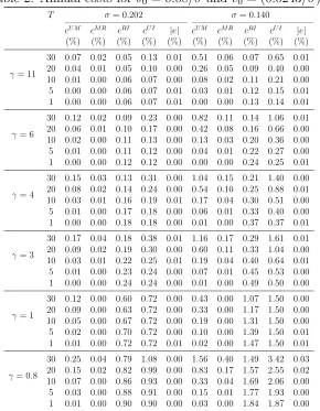
Table 2: Annual costs for θ0 = 0.08/σ and v0 = (0.0243/σ)2.
T σ= 0.202 σ= 0.140
cU M cM R cRI cU I |e| cU M cM R cRI cU I |e|
(%) (%) (%) (%) (%) (%) (%) (%) (%) (%)
γ= 11
30 0.07 0.02 0.05 0.13 0.01 0.51 0.06 0.07 0.65 0.01 20 0.04 0.01 0.05 0.10 0.00 0.26 0.05 0.09 0.40 0.00 10 0.01 0.00 0.06 0.07 0.00 0.08 0.02 0.11 0.21 0.00 5 0.00 0.00 0.06 0.07 0.01 0.03 0.01 0.12 0.15 0.01 1 0.00 0.00 0.06 0.07 0.01 0.00 0.00 0.13 0.14 0.01
γ= 6
30 0.12 0.02 0.09 0.23 0.00 0.82 0.11 0.14 1.06 0.01 20 0.06 0.01 0.10 0.17 0.00 0.42 0.08 0.16 0.66 0.00 10 0.02 0.00 0.11 0.13 0.00 0.13 0.03 0.20 0.36 0.00 5 0.01 0.00 0.11 0.12 0.00 0.04 0.01 0.22 0.27 0.00 1 0.00 0.00 0.12 0.12 0.00 0.00 0.00 0.24 0.25 0.01
γ= 4
30 0.15 0.03 0.13 0.31 0.00 1.04 0.15 0.21 1.40 0.00 20 0.08 0.02 0.14 0.24 0.00 0.54 0.10 0.25 0.88 0.01 10 0.03 0.01 0.16 0.19 0.01 0.17 0.04 0.30 0.51 0.00 5 0.01 0.00 0.17 0.18 0.00 0.06 0.01 0.33 0.40 0.00 1 0.00 0.00 0.18 0.18 0.00 0.01 0.00 0.37 0.37 0.01
γ= 3
30 0.17 0.04 0.18 0.38 0.01 1.16 0.17 0.29 1.61 0.01 20 0.09 0.02 0.19 0.30 0.00 0.60 0.11 0.33 1.04 0.00 10 0.03 0.01 0.22 0.25 0.01 0.19 0.04 0.40 0.64 0.01 5 0.01 0.00 0.23 0.24 0.00 0.07 0.01 0.45 0.53 0.00 1 0.00 0.00 0.24 0.24 0.00 0.01 0.00 0.49 0.50 0.00
γ= 1
30 0.12 0.00 0.60 0.72 0.00 0.43 0.00 1.07 1.50 0.00 20 0.09 0.00 0.63 0.72 0.00 0.33 0.00 1.17 1.50 0.00 10 0.05 0.00 0.67 0.72 0.00 0.19 0.00 1.31 1.50 0.00 5 0.02 0.00 0.70 0.72 0.00 0.10 0.00 1.39 1.50 0.01 1 0.01 0.00 0.72 0.72 0.01 0.02 0.00 1.47 1.50 0.01
γ= 0.8
Figure 4: Annual costs against investment horizon T (≤ 30) for σ = 0.202, θ0 =
investment horizon (in years)
annual costs (in percentage)
cUM
investment horizon (in years)
annual costs (in percentage)
cUM
investment horizon (in years)
annual costs (in percentage)
cUM
investment horizon (in years)
annual costs (in percentage)
cUM
investment horizon (in years)
annual costs (in percentage)
cUM
investment horizon (in years)
annual costs (in percentage)
Figure 5: Annual costs against investment horizon T (≤ 250) for σ = 0.202, θ0 =
investment horizon (in years)
annual costs (in percentage)
cUM
investment horizon (in years)
annual costs (in percentage)
cUM
investment horizon (in years)
annual costs (in percentage)
cUM
investment horizon (in years)
annual costs (in percentage)
cUM
investment horizon (in years)
annual costs (in percentage)
cUM
investment horizon (in years)
annual costs (in percentage)
Figure 6: Annual costs against risk aversion γ(≤12) forσ= 0.202,θ0 = 0.08/σ and
annual costs (in percentage)
cUM
annual costs (in percentage)
cUM
annual costs (in percentage)
cUM
annual costs (in percentage)
cUM
annual costs (in percentage)
cUM
annual costs (in percentage)
ascribable to the sole investment advisory services that do not include administrative services and overheads, for instance.
5
Conclusion
In this paper we evaluate the utility effects – in terms of additional fraction of initial wealth that makes two investment strategies indifferent – of two different degrees of bounded rationality for a CRRA investor operating in a continuous-time financial market with parameter uncertainty and compare them between each other and with the effect of uncertainty measured by the additional fraction of initial wealth that makes a rational agent indifferent between a full information and a partial informa-tion scenario. Agents may be boundedly rainforma-tional in that they either do not learn from fluctuations in the conditional distribution of the unobserved variable as more information come to light (myopic investors), or they completely disregard available information provided by prices and its predictable role (unconditional investors). The welfare difference between two different scenarios is quantified in terms of frac-tion of initial wealth needed to obtain the same expected utility. We find that, for reasonable values of the parameters, the main effects are produced, depending on risk aversion and investment horizon, by full information and/or predictability, being the effect of learning marginal.
We also investigate the saver’s decision of whether to manage her/his portfolio personally or hire, against the payment of a management fee, a professional investor. We find that delegation is mainly motivated, depending on risk aversion and invest-ment horizon, by the beliefs that professional investors are either better informed (“insiders”) or more capable of gathering and processing information rather than their ability of learning from financial data. In particular, for very short invest-ment horizons, we find the delegation is primarily, if not exclusively, motivated by the beliefs that professional investors are better informed. Moreover, it is also sug-gested that aggressive investors (i.e., γ < 1) are presumably the more interested in delegation.
It would be interesting to extend the analysis to more general settings in terms of utility functions and/or uncertainty structure. This is left for further research.
References
1051–1121. Elsevier Science B.V., 2003.
[2] T. Bj¨ork, M. Davis, and C. Land´en. Optimal investment under partial informa-tion. Mathematical Methods of Operations Research, 71:371–399, 2010.
[3] N. Branger, L. Larsen, and C. Munk. Robust portfolio choice with ambiguity and learning about return predictability. Journal of Banking and Finance, 37:1397– 1411, 2013.
[4] S. Brendle. Portfolio selection under incomplete information. Stochastic Pro-cesses and their Applications, 106:701–723, 2006.
[5] M. Brennan. The role of learning in dynamic portfolio decisions. European Finance Review, 1:295–306, 1998.
[6] M. Brennan and W. Torous. Individual decision making and investor welfare.
Economic Notes, 28:119–143, 1999.
[7] M. Brennan and Y. Xia. Persistence, predictability, and portfolio planning. In C.-F. Lee, A. Lee, and J. Lee, editors, Handbook of Quantitative Finance and Risk Management, pages 289–318. Springer, 2010.
[8] S. Browne and W. Whitt. Portfolio choice and the bayesian kelly criterion.
Advances in Applied Probability, 28:1145–1176, 1996.
[9] J. Cvitani´c, A. Lazrak, L. Martellini, and F. Zapatero. Dynamic portfolio choice with parameter uncertainty and the economic value of analysts recommenda-tions. The Review of Financial Studies, 19:1113–1156, 2006.
[10] W. De Bondt and R. Thaler. Financial decision-making in markets and firms: A behavioral perspective. In R. Jarrow, V. Maksimovic, and W. Ziemba, editors,
Handbooks in Operations Research and Management Science, Volume 9, pages 385–410. Elsevier, Amsterdam, 1995.
[11] M. Haugh, L. Kogan, and J. Wang. Evaluating portfolio policies: A duality approach. Operations Research, 54:405–418, 2006.
[12] T. Honda. Optimal portfolio choice for unobservable and regime-switching mean returns. Journal of Economic Dynamics and Control, 28:45–78, 2003.
[14] I. Karatzas and X. Zhao. Bayesian adaptive portfolio optimization. In E. Jouini, J. Cvitani´c, and M. Musiela, editors, Option Pricing, Interest Rates and Risk Management, pages 632–669. Cambridge University Press, 2001.
[15] Y. Kuwana. Certainty equivalence and logarithmic utilities in consump-tion/investment problems. Mathematical Finance, 5:297–310, 1995.
[16] P. Lakner. Utility maximization with partial information. Stochastic Processes and their Applications, 56:247–273, 1995.
[17] L. Larsen and C. Munk. Robust portfolio choice with ambiguity and learning about return predictability. Journal of Economics Dynamics & Control, 36:266– 293, 2012.
[18] M. Longo and A. Mainini. Learning and portfolio decisions forCRRAinvestors.
International Journal of Theoretical and Applied Finance, 19, 1650018, 2016.
[19] L. Pastor and P. Veronesi. Learning in financial markets. NBER Working Paper 14646, 2009.
[20] H. Pham. Portfolio optimization under partial observation: theoretical and numerical aspects. In D. Crisan and B. Rozovsky, editors,The Oxford Handbook of Nonlinear Filtering, pages 990–1018. Oxford University Press, 2011.
[21] U. Rieder and N. B¨auerle. Portfolio optimization with unobservable markov-modulated drift process. Journal of Applied Probability, 42:362–378, 2005.
[22] R. Rishel. Optimal portfolio management with partial observation and power utility function. In W. McEneany, G. Yin, and Q. Zhang, editors, Stochastic Analysis, Control, Optimization and Applications: Volume in Honor of W. H. Fleming, pages 605–620. Birkh¨auser Verlag, Boston, 1999.
[23] L. Rogers. The relaxed investor and parameter uncertainty. Finance and Stochastics, 5:131–154, 2001.
6
Appendix
We sketch the main steps in the derivation of indirect utilities (2.6), (2.14), (2.18) and (2.23). We treat the power case (i.e., γ 6= 1), the logarithmic case (i.e., γ = 1) can be treated similarly. Moreover, it can be proved that each logarithmic case is the limit of the power case asγ →1 (more precisely, for each i,Vi(x; 1, T) is the limit of
Vi(x;γ, T)−1/(1−γ), asγ →1). Recall the definition ˆΘ(t, y) = (θ
0+v0y)/(1 +v0t) (see (2.10)), hence ˆΘy = v0/(1 +v0t). Finally, in this appendix subscripts denotes partial derivatives.
6.1
Fully informed investors
Assume that at time 0 the agent observes Θ = θ, θ ∈ R, then he/she follows the standard Merton’s investment rule
π∗(t, θ) = θ
σγ, 0≤t ≤T, (6.1)
and enjoys an expected utility (cf. Rogers [23], Section 6)
v∗(x;θ) = x 1−γ
1−γ exp
r(1−γ)T + 1−γ 2γ θ
2T
. (6.2)
The expected utility (2.6) forγ 6= 1 is obtained by integrating over θ, that is
VI(x;γ, T) =
Z +∞
−∞
v∗(x;θ)p(θ)dθ, (6.3)
wherep denotes the Gaussian density with mean θ0 and variance v0.
6.2
Rational investors
The optimal investment policy (2.13) and expected utility (2.14) are derived by using dynamic programming techniques (cf., Karatzas and Zhao [14] or Rogers [23], Section 6). For each 0≤t≤T,x >0 and y∈R, let (see (2.12) and (2.9))
(
dXs =rXsds+σπ(s)Xs( ˆΘ (s, Ys)ds+dWˆs), Xt=x, t≤s≤T,
dYs= ˆΘ (s, Ys)ds+dWˆs, Yt=y, t≤s≤T,
(6.4)
and define the value function
vR(t, x, y) := sup
π∈At
1 1−γE
XT1−γ
where At is the set of all FS t
-progressively measurable and integrable controls
π = (π(s))s∈[t,T] such that (6.4) admits a unique solution. vR, under appropriate
regularity conditions, satisfies the Hamilton-Jacobi-Bellmann (HJB) equation
sup
γ). Assuming vxx < 0, the maximization on the LHS of (6.6) yields the following
candidate for the optimal (Markov) investment strategy:
π∗(t, x, y) = −Θ(ˆ t, y)vx
σxvxx
− vxy
σxvxx
. (6.7)
By substituting (6.7) into HJB (6.6), the latter reduces to:
vt+rxvx−
with the same boundary condition. For γ 6= 1, that is, the non-logarithmic case,15 we try solutions of the form:
v(t, x, y) = (xe
r(T−t))1−γ
1−γ h(t, y), (6.9)
h(t, y) = exp(a(t) ˆΘ2(t, y) +b(t) ˆΘ(t, y) +c(t)), (6.10)
a(T) =b(T) =c(T) = 0. (6.11)
The partial derivatives of v are:
vt =
Notice that any solution of the form (6.9) is such that vxx < 0. Substitute the
previous derivatives into (6.8) and get the following PDE forh:
ht
The partial derivatives of h can be written as follows:
ht = (a′Θˆ2+b′Θ +ˆ c′ −(2aΘ +ˆ b) ˆΘ ˆΘy)h,
hy = (2aΘ +ˆ b) ˆΘyh
hyy = ((2aΘ +ˆ b)2 + 2a) ˆΘ2yh.
where we use the identity ˆΘt = −Θ ˆˆΘy (see definition (2.10)). By substituting into
(6.12) and collecting the powers of ˆΘ, we have
0 = a′+2 ˆΘ
for each 0≤t≤T. Now, a standard verification argument proves
which, once substituted the optimal state dynamics, yields the optimal investment strategy (2.13). That is, πR
γ(t) =π∗(t, Xt, Yt).
6.3
Myopic investor
Substitute the myopic investment strategy (2.17) into (2.12) to get the state dynamics
Then, under appropriate regularity conditions, vM satisfies the PDE
vt+rxvx+
Forγ 6= 1, we proceed similarly to the rational case and try solutions of the form:
v(t, x, y) = (xe
r(T−t))1−γ
h(t, y) = exp(a(t) ˆΘ2(t, y) +b(t) ˆΘ(t, y) +c(t)), (6.20)
a(T) =b(T) =c(T) = 0. (6.21) The partial derivatives of v are as in the rational case and, once substituted into (6.18), yield the following PDE forh:
ht
Again, the partial derivatives ofh are as before and (6.22) becomes:
0 = a′+ 2 ˆΘ2ya2+ 2 (1−γ) ˆΘy
wherer1 < r2 are the roots of r2+ (2/γ−1)r+ (1−γ)/γ. Hence,
vM(t, x, y) = (xe
r(T−t))1−γ
1−γ exp(a
M
(t) ˆΘ2(t, y)+bM(t) ˆΘ(t, y)+cM(t)), γ 6= 1, (6.24)
for all 0≤t ≤T,x >0,y∈R, and the expected utility (2.18), forγ 6= 1, is obtained by fixingt = 0 and y= 0 in vM, that is
VM (x;γ, T) =vM(0, x,0) (6.25)
(notice thatϕM(γ, T) =aM(0) and ψM(γ, T) =cM(0) +r(1−γ)T).
6.4
Unconditional investors
Substitute the myopic investment strategy (2.22) into (2.12) to get the state dynamics
dXs=rXsds+
θ0
γ Xs( ˆΘ (s, Ys)ds+dWˆs), Xt =x, t≤s ≤T, dYs = ˆΘ (s, Ys)ds+dWˆs, Yt =y, t≤ s≤T.
(6.26)
Define
vU(t, x, y) := 1 1−γE
XT1−γ
. (6.27)
Then, under appropriate regularity conditions, vU satisfies the PDE:
vt+rxvx+
1
γΘ(ˆ t, y)θ0xvx+ ˆΘ(t, y)vy+ θ2
0 2γ2x
2v
xx+
θ0
γxvxy+
1
2vyy = 0, (6.28)
0 ≤ t < T, x > 0, y ∈ R, with boundary condition v(T, x, y) = x1−γ/(1−γ). For
γ 6= 1, we proceed as in the previous two cases and try solutions of the form:
v(t, x, y) = (xe
r(T−t))1−γ
1−γ exp(a(t) ˆΘ(t, y) +b(t)), (6.29)
a(T) =b(T) = 0. (6.30)
Computations similar to the previous two cases proves that v solves (6.28) if, and only if, the functionsa(t) and b(t) solve, for all 0≤t < T, the system of ODEs:
a′+1−γ
γ θ0 = 0
b′+ 1−γ
γ θ0Θˆya+
1 2Θˆ
2
ya2−
1−γ
2γ θ
2 0 = 0.
The solution that satisfies the terminal condition a(T) = b(T) = 0 is:
aU(t) = 1−γ
γ θ0(T −t),
bU(t) = (1−γ)(T −t) 2γ2
(1−γ)1 +v0T 1 +v0t
−1
θ20,
0≤t ≤T. Hence,
vU(t, x, y) = (xe
r(T−t))1−γ
1−γ exp(a
U(t) ˆΘ(t, y) +bU(t)), γ 6= 1, (6.32)
for all 0≤t ≤T,x >0,y∈R, and the expected utility (2.23), forγ 6= 1, is obtained by fixingt = 0 and y= 0 in vU, that is