Kirk Doran is an assistant professor in the department of economics at the University of Notre Dame. The author is grateful for helpful comments from Orley Ashenfelter, Anne Case, Marie Connolly, Angus Deaton, Susan Dynarski, Eric Edmonds, Henry Farber, Molly Fifer, Jane Fortson, Sergei Guriev, Daniel Hunger-man, Radha Iyengar, Alan Krueger, Giovanni Mastrobuoni, Christina Paxson, Jesse Rothstein, Cecilia Rouse, Derek Neal, Joseph Price, Analia Schlosser, Courtney Stoddard, Elod Takats, Chris Udry, Susan Yeh, and anonymous referees. He also warmly thanks Oportunidades for their kind permission to use the PROGRESA data. The data used in this article can be obtained beginning January 2014 through December 2016 from Kirk Doran, 438 Flanner Hall, Department of Economics, University of Notre Dame, kdoran@ nd.edu.
[Submitted November 2011; accepted August 2012]
SSN 022 166X E ISSN 1548 8004 8 2013 2 by the Board of Regents of the University of Wisconsin System
T H E J O U R N A L O F H U M A N R E S O U R C E S • 48 • 3
Demand for Adult Labor?
Evidence from Rural Mexico
Kirk B. Doran
A B S T R A C T
Do employers substitute adults for children, or do they treat them as complements? Using data from a Mexican schooling experiment, I fi nd that decreasing child farmwork is accompanied by increasing adult labor demand. This increase was not caused by treatment money reaching farm employers: there were no signifi cant increases in harvest prices and quantities, nonlabor inputs, or nonfarm labor supply. Furthermore, coordinated movements in price and quantity can distinguish this increase in demand from changes in supply induced by the treatment’s income effects. Thus, declining child supply caused increasing adult demand: employers substituted adults for children.
I. Introduction
loss that families face when some of their children are no longer working (Basu and Van 1998). If, however, adults and children are complements, then interventions that reduce child labor (such as discouraging the purchase of products produced by child labor) will reduce the demand for adult labor and thus reduce working households’ welfare. In this situation, interventions may need to be coupled with government trans-fers to compensate families for the drop in welfare.
Many of the policy proposals designed to reduce child labor assume that child and adult labor are substitutes. For example, the Child Labor Deterrence Act introduced in the United States in 1999 argues: “The employment of children under the age of 15 . . . ignores the importance of increasing jobs, aggregated demand, and purchas-ing power among adults as a catalyst to the development of internal markets and the achievement of broadbased, self- reliant economic development in many developing countries.” Likewise, the International Labor Organization’s book “Combating Child Labour,” claims that “ . . . child labour is a cause of, and may even contribute to, adult unemployment and low wages . . . ” (Bekele and Boyden 1988).
Despite these claims, the evidence that removing children from the work force im-proves adult labor market outcomes is sparse and contradictory, a point fi rst noted by Galli (2001) in her review of the literature. In his Handbook of Development Econom-ics chapter, Edmonds (2008) notes that whether child labor depresses adult wages “is a critical question in the child labor literature,” but that despite the critical nature of the question, “direct evidence on whether child labor affects adult labor markets is scarce.”1 In this paper, I address this empirical gap.
The reason for this gap is no surprise. Consider a simple production function with two inputs, A and B. The prices for the inputs are jointly determined, but an exogenous shock to the supply curve for input A will produce a corresponding change in the demand for B. The subsequent change in market conditions for input B will indicate whether the goods are complements or substitutes. But when we apply the model to a setting with child labor, we face a further complication. The two production inputs I consider (adult and child labor) come from the same household and, as a result, any program that changes child labor supply will almost certainly affect adult labor supply as well. Therefore, any test must allow for the possibility that the adult labor demand and supply curves are moving at the same time. My strategy, as developed in Section II, can identify changes in adult demand without assuming that adult supply has remained constant, by analyzing coordinated movements in price and quantity. As I outline below, given an exogenous reduction in child labor supply (that is, one without alternative causal pathways), if adult wages and employment both increase (decrease) then adult and child labor must be substitutes (complements). However, if adult wages and employment move in opposite directions, the joint co- movement
in adult supply and demand curves makes it impossible to determine the sign of the parameter of interest.
I apply this strategy using data from Mexico’s PROGRESA program, a conditional cash transfer experiment that produced large reductions in child farmwork participa-tion, as well as large unconditional increases in income for eligible families not on the relevant decision margins (Section IV). I then document a subsequent increase in both the quantity and wages of adult work, indicating that employers substituted adults for children (Section V), regardless of what happened to adult labor supply due to the unconditional income effects of the program. This increase in adult labor demand was not directly caused by alternative causal pathways: most importantly, there were no signifi cant treatment effects on the demand for the output of produc-tion, or on the supply of other inputs to production (Section VII). Furthermore, the wages of healthy nontreated adults living around children who stopped working also increased, suggesting that neither treatment- related health and nutrition increases nor health and nutrition spillovers were responsible for the increase in demand for adult labor (Section VII).
II. Conceptual Framework and Identi
fi
cation Strategy
Suppose that there are a large number of farms buying and selling in competitive input and output markets. Each farm has the following production function:
(1) Y = F(X1, ...,Xi, ...,XK)
where Y is the quantity of output and Xi is the quantity of Factor i used in production.
I assume that F is strictly concave and strictly increasing in each argument.2 Each
farm solves its production problem in two steps. First, it calculates how to minimize the total cost associated with the production of a given quantity Y of output. Second, it calculates the quantity of output that maximizes its profi ts.
Let wi be the strictly positive wage paid to Factor i. The cost minimization problem
can then be written as follows:
(2) Min
(X1,...,X K) w iXi
i=1 K
∑
subject to F(X1, ...,XK) ≥YThe Lagrangian associated with this problem is:
(3) L= (wiXi+ λ[F(X1, ...,XK)−Y]) i=1
K
∑
I defi ne Fi to be the partial derivative of F with respect to its ith argument. The fi rst order conditions are thus:
(4) ∂L
∂Xi = w
i+ λF
i = 0, ∀i=1, ...,K
Because wi and F
i are strictly positive, the production constraint is binding. Because
F is strictly concave, these necessary conditions for optimality are also suffi cient con-ditions for optimality. The fi rst order conditions and the binding production constraint produce the conditional factor demands: Xi. The cost function is defi ned as the
mini-mum value of the total cost given output Y and factor prices, or C(w1, ...,wK,Y).
Given these defi nitions, it is easy to show that the cost function satisfi es Shephard’s Lemma:
(5) Xi = Ci(w1, ...,wK,Y), ∀
i=1, ...,K
I defi ne adult workers to be Factor 1 and child workers to be Factor 2. I can then obtain an expression for the effect of a change in the wage of child workers (w2) on
the unconditional demand for adult workers (X1), by taking the derivative of Equation
5 with respect to w2, allowing both the optimal output Y and the demand for other
factors to adjust to the new price of child labor:
(6) ∂X1
A priori, the sign of Equation 6 is unknown. If there are only two inputs, then the fi rst term of Equation 6 is necessarily greater than zero; else, its sign is indeterminate. In either case, the sign of Equation 6 is undetermined theoretically, and I must apply an identifi cation strategy to empirical data in order to identify its sign in any given setting.
A. Basic Identifi cation Strategy
Based on Equation 6 and the definitions of gross- substitutes and gross- complements above, it is clear that the foundation of the identification strategy will be to ob-serve an exogenous change in X2 and w2 and a response to this change in the
function X1.
The Journal of Human Resources
Figure 1
707
increase in wages and quantities means that adult labor demand must have increased, and thus adult labor and child labor are substitutes.3
A similar story is outlined in the second row of fi gures in Figure 1. If the wages and employment of adults fall when children leave the work force, then it must be the case that adult and child labor are complements. In this case, regardless of the movement in labor supply, the demand curve must have shifted in. The story is not defi nitive, however, if wages and quantities move in opposite directions. Consider the third row of fi gures. In this case, a decline in the supply of child labor increases adult wages but reduces the quantity of adult labor. The fi gures in this row show that this change in equilibrium could be generated either by an increase in supply and a drop in demand (the third graph in the row) or a drop in supply and an increase in the demand for adult labor. Therefore, if wages and quantities move in opposite directions, we cannot say defi nitively without further data whether adult and child labor are complements or substitutes.
In the next subsections, I consider whether equilibrium in other factor markets and the output market imply any testable predictions that can be used to distinguish be-tween the gross- complementarity or the gross- substitutability of children and adults.
B. Accounting for the Supply of other Factors
If the supply of a third factor changed, then I cannot determine whether the observed sign of the change in X1 came from the change in the supply of child labor, or from the
change in the supply of the third factor. In other words, ∂X1/∂w2 could be negative or
positive without affecting the sign of the observed change in X1, if the magnitude of
∂X1/∂w3 was suffi ciently large. Therefore, I will also need to check whether the
sup-plies of other factors remained constant. In the absence of other information, the only way to be sure of this is to check the price and quantity of each of the other inputs and measure whether they each remained constant. If so, it is not possible that their sup-plies changed.
C. Accounting for the Farms’ Zero Profi t Condition
A change in the wage of children (denoted by ∆w2) will potentially affect the
equilib-rium in the other factor markets. In the long run, the change in the price of output, ∆p, must satisfy the following equation:
(7) ∆p= θi⋅ ∆wi i=1
K
∑
, where θi = the cost share of Factor iIn this agricultural setting, the price of corn is likely set on a world market; in any case, it is not altered by the treatment in comparison with nontreated villages (as I show later empirically). Thus ∆p will be 0 in the equation above. Using this fact, it is clear that if ∆w2 and ∆w1 are both positive (as would be the case if adults are
tutes with children and the supply of children decreases), then it is necessarily the case that ∆w3 should be negative for some third factor.
Technically, this does not introduce another testable prediction. Rather, this conclu-sion is drawn from an equation that is only required to hold in long- term equilibrium. In the short- term, fi rms can and will produce output at prices that exceed average vari-able cost but are exceeded by average total cost, thus breaking the equality of Equation 7. Since the relative decrease in child labor supply in my data covers only the period of one or at most two harvests, it is impossible to rule out that short- term effects will dominate, leaving the prices of third factors potentially unchanged by the increase in child wages. Nevertheless, it is likely that the demand for at least one other factor must decrease. I discuss the empirical evidence for this, and the implications for my identifi cation, in Section VIIB.
D. Accounting for the Supply and Demand of Output
If the fact that children and adults are gross- substitutes (or gross- complements) has a necessary implication for the supply of output, then this implication would have to be checked in a complete identifi cation strategy, and if it were verifi ed, it would serve as a useful piece of evidence for my conclusion. Rearranging terms in Equation 6 clearly shows that the sign of ∂X1/∂w2 does not determine the sign of ∂Y /∂w2. Likewise the
fact that w2 increases or decreases does not in itself imply anything about the direction
of any changes in the marginal cost schedule, or hence the direction of any changes in
Y when prices are held constant. This implies, of course, that general equilibrium ef-fects on the supply of output are ambiguous.
However, exogenous changes in the demand for output can obscure my identifi ca-tion in an analogous way to that specifi ed in IIIC above. Thus, I must rule out any changes in the demand for output. This requires verifying that the price and quantity of output remained the same.
E. Summary
I summarize the identifi cation strategy as follows: First, I must observe a decrease in the supply of child labor due to some treatment. Second, I must observe the price and quantity of adult labor moving in the same direction in the areas in which child labor has been treated. Third, I must observe constant price and quantity of output. Fourth, I must observe constant price and quantity of key “third” factors of production (allow-ing for the probability of a simultaneous decrease in price and quantity of at least one other factor of production).
III. Data
conditional on their children’s school attendance, school attendance would increase in the treatment group. Census and administrative data identifi ed 506 villages in rural Mexico as “poor” (Skoufi as and Parker 2001). Of these villages, 320 were randomly selected to form the treatment group. The remaining 186 villages formed the random-ized control group.4
Five surveys were conducted over households in all 506 villages at the following times: October 1997, March 1998, October 1998, May 1999 and November 1999. In the spring of 1998, the Mexican government announced that it would give benefi ts (conditional on children’s school attendance and family participation in health and nutrition programs) to the eligible families of the treatment group. The fi rst payments were made in May 1998. Thus, the fi rst two surveys are pretreatment, and the latter three surveys are during the treatment. After the experimental phase was complete, eligible control families began receiving benefi ts as well.
PROGRESA administrators used the results of the October 1997 census to deter-mine, based on variables associated with household welfare, the families that were relatively poor. It assigned these families to the eligible group, assigning relatively well- off families to the noneligible group (Skoufi as, Davis, and Behrman 1999). This assignment was conducted for families in both control and treatment villages. Eli-gible families in the treatment group of villages received conditional benefi ts targeted toward improving education and health; many eligible families not on the relevant decision margins experienced large unconditional increases in their income.5 If a child
younger than 18 missed fewer than 15 percent of the school days in a particular month, then PROGRESA provided a cash award that month to the mother of the child. Cash awards increased to keep pace with infl ation, increased with the child’s grade, and were higher for girls than boys. These monthly grants ranged from about 80 pesos for third graders to 280 pesos for ninth grade boys and 305 pesos for ninth grade girls. As a comparison, in 1997 the average monthly salary income of an adult farmworker was about 600 pesos, and that of a child farmworker was about 500 pesos. The program also provided basic healthcare for all family members and a fi xed monetary transfer for nutritional supplements (Skoufi as and Parker 2001).
I make use of data from this experimental phase of PROGRESA. I obtained the data from the Opportunidades offi ce. I primarily make use of three surveys that were conducted at the same time in the agricultural cycle (October / November): the pretreat-ment survey in 1997 and two posttreatpretreat-ment surveys in 1998 and 1999. The 506 vil-lages in the experiment were located in seven Mexican states in south central Mexico. When locals in each village were asked about their village’s principal activity and principal crop, 97.8 percent said agriculture and 88.2 percent said corn. The primary corn harvest in Mexico lasts from October through December (USDA), although a smaller corn harvest occurs in the summer. Thus, I interpret my results as information about production technology and labor demand during the primary corn harvest.
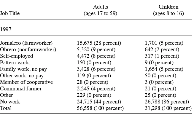
Table 1 shows the distribution of adults and children across the job categories listed in the main job category variable (one that is available each year). Workers in two job types consistently report salary information: jornaleros (farmworkers), and obreros
4. See Behrman and Todd (1999) for a discussion of the randomization procedure.
(nonfarmworkers)—those in other categories typically do not report earning a salary. This paper analyzes the jornalero work force, which has nearly three times as many observations as the obrero, and—given the corn- heavy nature of agriculture in this sample—is presumably more homogenous than the obrero work force (which seems to potentially include all regularly paid nonagricultural jobs).
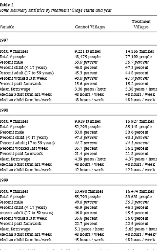
Table 2 reports summary statistics for important variables across both treatment and control villages over the three years in my sample: whether individuals were eligible for the program, whether they were working for a salary, what their job title was, mea-sures of their income, and meamea-sures of the amount of time they worked.
I classify people who are ages 16 and younger as children and people ages 17 to 59 as adults (I have also rerun all the subsequent results with 16 year- olds defi ned as adults, and none of them change appreciably). Children are a substantial portion of the farmwork force: in 1997, children made up 9 percent of the total farmwork force, while adults made up an additional 80 percent, and this holds with weighting by hours worked per week. I have tried to measure the sensitivity of my results to changes in the defi nitions of these age groups, and I have found the results to be robust.
Everyone who reports income reports it in one of the following measures: pesos per day, pesos per week, pesos per two weeks, pesos per month, or pesos per year. The measures of the amount of time worked are hours per day and days per week, and most people who report income report the amount of time they worked using both of these measures. About 90 percent of the income observations are in pesos per day or pesos per week. For people who report daily salaries, I impute hourly wages by dividing the daily salary by the number of hours worked per day. For people who report weekly earnings, I impute hourly wages by dividing earnings by the number of days worked
Table 1
Pretreatment (1997) distribution of adults and children across job categories
Job Title
Adults (ages 17 to 59)
Children (ages 8 to 16)
1997
Jornalero (farmworker) 15,675 (28 percent) 1,701 (5 percent)
Obrero (nonfarmworker) 5,320 (9 percent) 642 (2 percent)
Self- employed 4,472 (8 percent) 317 (1 percent)
Pattern work 150 (0 percent) 9 (0 percent)
Family work, no pay 3,428 (6 percent) 1,654 (5 percent)
Other work, no pay 119 (0 percent) 50 (0 percent)
Member of cooperative 28 (0 percent) 3 (0 percent)
Communal farmer 2,245 (4 percent) 21 (0 percent)
Other 229 (0 percent) 25 (0 percent)
No work 24,715 (44 percent) 26,788 (86 percent)
Total 56,558 (100 percent) 31,298 (100 percent)
Table 2
Some summary statistics by treatment village status and year
Variable Control Villages
Treatment Villages
1997
Total # families 9,221 families 14,856 families
Total # people 48,475 people 77,199 people
Percent male 50.0 percent 50.7 percent
Percent child (< 17 years) 46.8 percent 47.3 percent
Percent adult (17 to 59 years) 45.3 percent 44.8 percent
Percent worked last week 40.0 percent 41.9 percent
Percent paid farmwork 15.6 percent 15.2 percent
Mean farm wage 3.36 pesos / hour 3.38 pesos / hour
Median adult farm hrs / week 48 hours / week 48 hours / week
Median child farm hrs / week 48 hours / week 48 hours / week
1998
Total # families 9,919 families 15,927 families
Total # people 52,299 people 85,141 people
Percent male 50.0 percent 50.6 percent
Percent child (< 17 years) 47.5 percent 48.1 percent
Percent adult (17 to 59 years) 44.7 percent 44.1 percent
Percent worked last week 35.7 percent 36.2 percent
Percent paid farmwork 21.4 percent 21.8 percent
Mean farm wage 4.39 pesos / hour 4.37 pesos / hour
Median adult farm hrs / week 48 hours / week 48 hours / week
Median child farm hrs / week 42 hours / week 42 hours / week
1999
Total # families 10,498 families 16,474 families
Total # people 55,793 people 83,631 people
Percent male 49.6 percent 50.3 percent
Percent child (< 17 years) 45.9 percent 46.3 percent
percent adult (17 to 59 years) 46.0 percent 45.5 percent
Percent worked last week 35.6 percent 36.0 percent
Percent paid farmwork 22.7 percent 22.5 percent
Mean farm wage 5.1 pesos / hour 5.65 pesos / hour
Median adult farm hrs / week 48 hours / week 48 hours / week*
Median child farm hrs / week 45 hours / week 48 hours / week
per week multiplied by the number of hours worked per day. For the remaining 10 percent of income observations, I assume that biweekly reporters work both weeks, that monthly reporters work four weeks per month, and that yearly reporters work fi fty weeks per year.
The resulting hourly wages range from 0.0003 pesos per hour to 7,506 pesos per hour. With bounds this extreme, it is likely that the very high and very low hourly wages suffer from measurement error. Mean regressions of wages are thus likely to be biased by the incorrect measurements at the top of the distribution, and mean regres-sions of log wages may be biased by the incorrect measurements at the bottom of the distribution. Thus, in later sections I will often perform two tests that do not depend only on means in order to establish the existence and direction of any treatment ef-fect on the distribution of wages: a Kolmogorov Smirnov test of fi rst- order stochastic dominance and estimation of quantile regressions by decile. But I do run mean regres-sions as well, attempting to eliminate the bias caused by the incorrect measurements at the top and the bottom of the distribution by dropping observations with wages in the top and bottom 5 percent for each of the six comparison groups (control vs. treatment, 1997 vs. 1998 vs. 1999).6
The setting described by this data is highly policy- relevant, since corn production in Mexico in the late 1990s is quite representative of what we know about the modal child worker’s occupation. Regarding occupations, Edmonds (2008) reports in the Handbook of Development Economics that “in almost every listed country, a majority of economically active children are involved with agriculture, forestry, or fi shing in-dustries.” Edmonds explains further that: “Children involved in agriculture and related industries are involved in the growing of cereals, vegetables, poultry farming, and inland fi shing. Cereal cultivation is the largest single sector with 39 percent of all eco-nomically active children directly involved.” Edmonds writes as well: “Information at the 3 digit level is available in the Bangladesh child labor force survey, . . . 46 percent of children 5–17 are farm crop workers. The next largest occupations are salesmen and shop assistants (7 percent), poultry farmers (5 percent), sales supervisors (4 percent),
fi sherman (3 percent), and nonmotorized road vehicle drivers (3 percent).”
Finally, farm households in south- central Mexico in the late 1990s had access to machinery that would help in production, harvesting, and transport of corn. In PRO-GRESA’s October 1998 household survey, about 15 percent of the land was controlled by households that owned one or more of the following types of equipment: a truck or van, a tractor, a thresher, a sprayer or pump, or a windmill. This is a larger percent-age than the percentpercent-age of households whose children worked for pay in the fi elds. Furthermore, this percentage vastly underestimates the percentage of smaller house-holds that rent the richer househouse-holds’ threshers and other equipment for the duration of their harvest, as is common in areas with many small farms. Thus, this is a setting in which there is suffi cient capital to switch technology and introduce less labor- intensive means of production.
IV. Did the Experiment Reduce the
Supply of Child Labor?
In the fi rst few months of the program, as measured by the 1998 sur-vey, it is unclear whether the experiment has yet reduced the supply of children to the farmwork force. But by 1999, 18 months after the program started, the treatment has clearly caused a decline in child participation in the farmwork force as well as an increase in the wages of child farmworkers. These results are demonstrated in the difference- in- difference estimates of the treatment effect described below.
My primary empirical strategy is to estimate reduced form equations of the treatment effects on labor market outcomes such as work participation, hourly wages, etc. The unit of observation is an individual at a point in time. I use a difference- in- difference approach to address the small ways in which treatment and control villages differed before the treatment even started as well as to control for persistent sources of regional variation (Schultz 2004). I also control for individual- level characteristics and cluster the standard errors at the village level in most specifi cations.
Thus, in summary, the difference- in- difference equations are of the following pat-tern:
(8) Yit = (α ⋅Pt⋅Ei)+(β ⋅Pt)+(γ ⋅Ei)+(δ ⋅Xit)+εit
Where Pt is an indicator for posttreatment, Ei is an indicator for a treatment village, and Xit is a vector of personal characteristics; i indexes people (or households, depend-ing on the case), and t indexes time.
I include in Xit dummies for gender, age, schooling, language abilities and marriage status (where these are age- and specifi cation- appropriate).7 I run this specifi cation
separately for the 1997 vs. 1998 comparison and the 1997 vs. 1999 comparison. When the dependent variable was not recorded in the pretreatment survey, then I cannot include the Pt dummy (because it is always 1) or the Pt • Ei dummy (because it always equals the Pt dummy). Thus, the coeffi cient on the Ei dummy becomes my estimate of the treatment effect, and my estimation equation becomes:
(9) Yit = (γ ⋅Ei)+(δ ⋅ Xi)+ εi
where i indexes people (or households) and t indexes time.
In specifi cations based on Equation 9, I cannot control for village- level fi xed ef-fects, because that would require me to omit the Treatment Village dummy.
I add to the previous studies of this experiment (such as Schultz 2004, Skoufi as and Parker 2001) that estimated signifi cant decreases in work participation for children, by estimating specifi cally the treatment effect on child participation in the farmwork force. I create a dependent variable dummy for working on a farm by assigning the dummy the value 1 if the person worked on a farm for pay in the last week and 0 if they did not work or worked in a different job category. I regress the dummy for work-ing on a farm on my independent variables as outlined in Equation 1. Table 3 reports the results of probit specifi cations of this regression model. I fi nd that by 1998, there
Doran
Difference- in- Difference –0.002 –0.002** –0.009 –0.014** (post = 1 & treatment
Number of observations 61,127 58,851 50,190 61,228
Pseudo R2 0.33 0.36 0.21 0.29
The unit of observation is an individual child (a person aged less than 17). Specifi cation 1 includes years 1997 (pretreatment) and 1998 (posttreatment). Specifi cations 2 through 4 include Years 1997 (pretreatment) and 1999 (posttreatment). Coeffi cients reported are the marginal effects calculated from the probit coeffi cients. The estimated equation is Equation 8 in Section IV, with age dummies and village- level fi xed effects. The difference- in- differences coeffi cient is interpreted as a percentage change in the row “Treatment Effect Percentage Change,” by dividing the difference- in- difference coeffi cient by the percentage of children for whom the dependent variable is 1 in the pretreatment survey. Standard errors, adjusted for village- level clustering, are in parentheses.
was no signifi cant effect on child- paid farmwork participation. However, by 1999, paid child farmwork participation saw a signifi cant decrease of 4 percent due to the treatment.8 When I extend my defi nition of child labor to a broader measure of work,
I fi nd an even larger effect of 12 percent.9
I include both eligible and ineligible children in the specifi cation because I am interested in the program effects on overall child wages and quantities (note that the ineligible children in treatment villages likely increased their labor supply in response to the wage increase, so the treatment’s impact on eligible children’s labor supply is likely larger than what I report in this specifi cation).
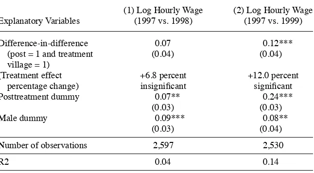
If the supply schedule of child farm labor slopes upward, then one can always tell that the supply schedule has shifted backward (decreased) when a decrease in the quan-tity of child farm labor is accompanied by an increase in the price of child farm labor. Thus, in Table 4, I report the results of OLS estimation of the difference- in- difference treatment effects on child hourly wages. It is clear that the treatment has caused a large increase in mean child hourly wages, and that this increase is statistically signifi cant. This wage increase necessarily implies a decrease in the supply of child farmworkers. Even if the magnitude of the wage increase is infl ated because of selection (as one would expect given the large magnitude), selection of low- productivity children out of the work force presupposes a decline in the supply of child workers (whose quan-tity effect is seen in Table 3). Thus, nothing other than a decline in child labor supply succinctly explains the participation results in Table 3 coupled with the wage results in Table 4.
V. Was there an Increase in the
Demand for Adult Labor?
Because the results in the previous section showed that there was a decrease in child labor supply to the farmwork force by 1999, I need to check whether the demand for adult labor increased by 1999 as well.10 If the treatment increased
the price of adult farm labor without decreasing its quantity (or vice versa), then this implied that it increased the demand for the labor of adult farmworkers.
The Kolmogorov Smirnov test on the pretreatment distribution functions shows that
8. The percentage change is calculated by dividing the coeffi cient on the Difference-in-Differences dummy from Table 5 by the pretreatment mean value of the independent variable, 0.054.
9. According to Table 3, children classifi ed as either working for their families without payment or self-employed make up almost all of the working children who are not paid farmworkers. According to the May 1999 time-use supplement, these children work more than 10 times as many hours in their own family’s fi elds than other children do. Thus, it is relevant to consider treatment effects on the broader measure of child farm labor that includes both paid farmworkers and these other workers who work so much in their own family’s fi elds. I do so in Specifi cation 4 of Table 3: This broader measure of child farmwork shows an even larger decline due to the treatment.
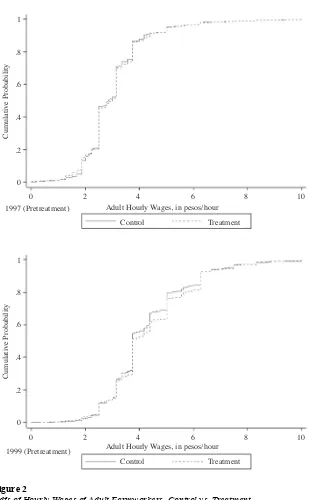
the pretreatment distribution of wages in treatment villages is fi rst- order stochastically dominated by that in the control villages. The p- value for the null hypothesis that the two distributions are identical—when the alternative hypothesis is that the treatment distribution is stochastically dominated by the control distribution—is 0.02, and is thus rejected. The p- value for the null hypothesis that the two distributions are identi-cal—when the alternative hypothesis is that the control distribution is stochastically dominated by the treatment distribution—is 0.20, and cannot be rejected.
But the Kolmogorov Smirnov test clearly shows that the posttreatment distribution of wages in the treatment villages fi rst- order stochastically dominates that in the con-trol villages. The p- value for the null hypothesis that the two distributions are identi-cal—when the alternative hypothesis is that the control distribution is stochastically dominated by the treatment distribution—is 0.00, and is thus rejected. The p- value for the null hypothesis that the two distributions are identical—when the alternative hypothesis is that the treatment distribution is stochastically dominated by the control distribution—is 0.38, and cannot be rejected.
This shift can be seen visually in Figure 2, which plots the cumulative distribution functions of the hourly wages of adult farmworkers in 1997 and in 1999. The wage distribution is too lumpy for all deciles to increase, but the quantile regressions by
Table 4
Treatment effects on hourly wages of child farmworkers
Explanatory Variables
Number of observations 2,597 2,530
R2 0.04 0.14
The unit of observation is an individual child farmworker (a person aged less than 17). Specifi cation 1in-cludes years 1997 (pretreatment) and 1998 (posttreatment). Specifi cation 2 includes years 1997 (pretreat-ment) and 1999 (posttreat(pretreat-ment). Coeffi cients reported are the marginal effects from a linear regression model with village- level fi xed effects. The estimated equation is Equation 8 in Section IV. Both specifi cations in-clude dummy variables for each year of age, and village- level fi xed effects. The difference- in- differences coeffi cient is interpreted as a percentage change in the row “Treatment Effect Percentage Change.” Standard errors, adjusted for village- level clustering, are in parentheses.
1997 (Pretreatment) Adult Hourly Wages, in pesos/hour Control Treatment
Cumulative Probability
1
.8
.6
.4
.2
0
0 2 4 6 8 10
1999 (Pretreatment) Adult Hourly Wages, in pesos/hour Control Treatment
Cumulative Probability
1
.8
.6
.4
.2
0
0 2 4 6 8 10
Figure 2
decile reported in Table 5 show that three deciles experienced large and signifi cant increases (two below the median and one above) and none decreased signifi cantly.
It is clear that by 1999 the hourly wages of adult farmworkers have increased due to the treatment. Furthermore, the adult wage increase appears to be real, not only nominal: the study by Handa et al. (2000) concludes that the treatment did not produce food price infl ation in the treated villages. I further consider the treatment’s effect on mean wages by estimating OLS regressions on log hourly wages and log daily income according to Equation 8 (with the effect of the tails diminished via the cropping dis-cussed in Section III), reporting the results in Table 6, Specifi cations 1 and 2. There is an increase in mean adult farm wages of about 3 percent. I also estimate treatment effects on mean work outcomes for adults. From Table 6, Specifi cations 3 and 4, it is clear that the treatment increased both adult hours worked per week and adult days
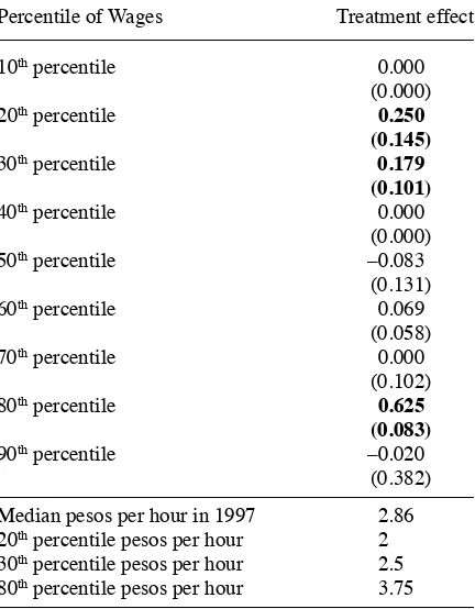
Table 5
Quantile difference- in- difference treatment effects on hourly wages of adult farmworkers, 1997 vs. 1999
Percentile of Wages Treatment effect
10th percentile 0.000
(0.000)
20th percentile 0.250
(0.145)
30th percentile 0.179
(0.101)
40th percentile 0.000
(0.000)
50th percentile –0.083
(0.131)
60th percentile 0.069
(0.058)
70th percentile 0.000
(0.102)
80th percentile 0.625
(0.083)
90th percentile –0.020
(0.382)
Median pesos per hour in 1997 2.86
20th percentile pesos per hour 2
30th percentile pesos per hour 2.5
80th percentile pesos per hour 3.75
The Journal of Human Resources
Table 6
Treatment effects on adult farmworkers, from 1997 to 1999
Explanatory Variables
(1) Log Hourly Wage
(2) Log Daily Income
(3) Log Hours per Week
(4) Log Days per Week
(5) Paid Farmwork
Difference- in-difference (post 0.032* 0.028 0.033* 0.037** 0.011 = 1 and treated village = 1) (0.019) (0.019) (0.019) (0.017) (0.014) (Treatment percentage change) + 3.2 percent
signifi cant
+ 2.8 percent insignifi cant
+ 3.3 percent signifi cant
+ 3.7 percent signifi cant
+ 4.1 percent insignifi cant Treatment village indicator –0.010 –0.001 –0.030* –0.039*** –0.004
(0.022) (0.022) (0.016) (0.015) (0.015) Posttreatment indicator 0.327*** 0.316*** –0.073*** –0.059*** 0.061***
(0.014) (0.014) (0.014) (0.012) (0.011) Male indicator 0.026** 0.051*** 0.097*** 0.072*** 0.554***
(0.012) (0.012) (0.016) (0.015) (0.009)
Constant 1.08*** 3.12*** 3.60*** 1.56***
(0.026) (0.027) (0.025) (0.002)
Number of observations 26,290 26,290 26,254 26,254 103,385
R2 0.26 0.26 0.35 0.33 0.34
The unit of observation is an individual prime- age adult farmworker (a person aged 17 through 59). Observations are dropped at the tails of the wage distribution according to the cropping rules discussed in Section III. Coeffi cients reported in Specifi cations 1 through 4 are the marginal effects from a linear regression model, controlling for gender, age dummies, schooling level, language skills, and marriage status. The coeffi cients reported in Specifi cation 5 are the marginal effects from a probit regression model. The estimated equation is Equation 8 in Section IV. Standard errors, corrected for village- level clustering, are in parentheses.
worked per week conditional on working. Finally, Table 6, Specifi cation 5 shows that the treatment did not decrease the probability of adult participation in the farmwork force. The fi rst four specifi cations in Table 6 have standard errors that are sensitive to the degree of cropping of the tails of the wage distribution, as well as to controls for village- level fi xed effects.11
It is instructive to consider how the program may have had different labor supply effects for different groups of adults, and what the implications of this would be for identifi cation of a labor demand shift. Specifi cally, some low- productivity adults may have decreased their labor supply while other adults may have increased their labor supply. In general, if there are two groups within the adult labor pool, and if the high- productivity group faces a very elastic demand curve, and if the high- productivity group increases its labor supply by more than the low- productivity group, then it is defi nitely the case that the quantity of labor would increase. And if this quantity in-crease happened at the extensive margin, then the average wage would inin-crease as well (if it didn’t happen at the extensive margin, then the fact that I am estimating wages in a “one person, one observation” setting means that average wages would not go up). This simultaneous increase in price and quantity could therefore happen where labor demand has stayed constant, as long as each of the assumptions above is satisfi ed.
This alternative hypothesis affects mean wages, due to a composition effect on the extensive margin. My decile regressions are therefore useful here. Under the scenario above, the wage increase is entirely an artifact of a changing labor pool in which high- productivity people have out- numbered low- productivity people. This should increase the levels of each wage percentile at all percentiles below the one in which we have added workers. Importantly, though, this should decrease the levels of each wage percentile at all percentiles above the one in which we have added workers. But the quantile difference- in- differences regressions in Table 5 show that the 80th percentile increased substantially (as well as the 20th and the 30th), and that none decreased signifi cantly, including the 90th percentile. Thus, increasing the relative number of high- productivity people can’t explain the observable changes in the full- wage distribution from top to bottom. Furthermore, the assumption that all demands for labor are strictly downward- sloping implies that increasing the labor supply of high- productivity people should substantially decrease the levels at the highest wage percentiles, meaning that this alternative hypothesis disagrees signifi cantly with the observable changes in the empirical wage distribution.
There is another empirical implication of this composition bias story: In order for changes in composition of the work force to have affected mean wages, the participa-tion rates of highly productive adults must have increased more than the participaparticipa-tion rates of adults with less than mean productivity. To test this implication, I run addi-tional regressions on participation of prime- age adults in farm day labor by schooling category. Breaking the schooling variable into two categories of roughly equal size (low and high), I observe that the wages of the low category are less than the mean
wages overall, and the wages of the high category are greater than the mean wages overall. Thus, schooling is a useful proxy for productivity. Running regressions of farmwork on the extensive margin, I fi nd that the low- productivity group had a large and signifi cant 7 percent increase in participation rates in farm labor, while the high- productivity group had a much smaller and statistically insignifi cant change of less than 1 percent. Thus, there is no evidence of increased relative work in the extensive margin for high- skilled workers. In fact, any composition bias is pushing downward my observed wage increase from what it would have been without a composition change.
Taken together, both the effects on the wage distribution and the participation re-sults suggest that composition bias is not at work in this wage increase. Rather, the combined increase in price and quantity of adult farm labor implies that the demand for adult labor must have increased.
VI. Comparison of the Size of the Effects
Table 3 shows that the reduction in the number of child farmworkers was anywhere from – 4 percent (for the most restrictive defi nition of child farmwork-ers) to –12 percent (for the broadest defi nition of child farmworkers). Children made up 9 percent of the paid farmwork force, and 12 percent of the broadest defi nition of farmworkers. Thus, this reduction in the number of child farmworkers amounted to a reduction in the total number of farmworkers of anywhere from – 0.3 percent (using the most restrictive defi nition of farmworkers) to –1.4 percent (using the broadest defi nition).
It is reasonable that a –1.4 percent decrease in the total quantity of labor could cause a +3 percent increase in the price of labor among at least one set of substitutable workers. It is also reasonable that when 1.4 percent of the work force stops working, some remaining workers will have to work 3 percent more hours per week (as reported in Table 6).
Finally, the total number of hours of farmwork lost due to decreasing child farm-work participation has a similar order of magnitude to the total number of hours of farmwork added by adult farmworkers. Child farmworkers worked an average of 43 hours per week in the pretreatment data. Thus, a 12 percent reduction in the number of child farmworkers could account for as much as 5.2 fewer farm hours per week per child. A 3.3 percent increase in the hours of adult farmwork per week (Table 6) accounts for 1.4 more farm hours per week per adult. Rescaling by the larger number of adult farmworkers, this amounts to 11.3 additional adult hours per week per child farmworker. Accounting for the large standard errors in Table 6, this is a number well within the range of 5.2 fewer child farm hours per week per child farmworker.12
At the end of the next section I show that some of the impact on adult workers is due to health and nutrition benefi ts. In particular, I show that the impacts that remain when I account for health and nutrition benefi ts are still positive, though likely of a
smaller magnitude that is more similar to the magnitude of the reduction in overall labor supply caused by the child labor supply shock.
VII. Did the Reduction in Child Labor Cause the
Increase in the Demand for Adult Labor?
I explained in Section II that in order to determine whether adults and children are gross- substitutes or gross- complements, it is necessary to ensure that the treatment’s only effect on the demand for adult farm labor was through the decrease in child labor supply—or, rather, that there is still an effect on the demand for adult farm labor even when all nonchild pathways have been accounted for. There are four alter-native pathways to consider. One is that the treatment families spent their money in a way that would increase the demand for output, thus increasing the derived demand for the farmworkers’ labor. The second is that the treatment caused a change in the supply of other factors of production, which in turn caused an increase in the demand for adult farm labor (these fi rst two alternative pathways were considered theoretically in Section II). The third alternative pathway is that the direct treatment benefi ts in income, nutritional consumption, or medical consumption lead to improved health for those who received them, thus leading to better productivity and hence to better adult wages.13 The fourth is that the indirect treatment benefi ts (for example, spillovers in
income, nutritional consumption, or medical consumption) lead to improved health, leading to better productivity and hence to better adult wages. I rule out each of these four alternative pathways as the sole causes of the increase in adult demand below.
A. Ruling Out an Increase in Derived Demand
The program has many components that could plausibly affect nonfarm markets. Any of these effects on nonfarm markets could circle back to the farm labor market through changes in derived demand: that is, a change in the demand for the products produced by farm labor. For example, the income transfer aspects of the program are likely to directly increase the consumption of local families; some of this increase may be spent on local farm products. Likewise, the program should directly increase the demand for schooling and services related to the provision of schooling. This could increase the demand for construction labor, as well as the demand for meal provision and transport, in turn increasing the consumption of local farm products. The component to provide healthcare to treatment villages may have lead to increased hiring of local labor as well, with a subsequent effect on the demand for local farm products.
The fi rst thing to note is that an increase in the demand for adult labor in nonfarm industries cannot directly affect the demand for adult labor in farms. Rather, what the increase in demand for adult labor in nonfarm industries directly affects is the supply
of adult labor to farms. The way in which an increase in demand for adult labor in nonfarm industries affects the demand for adult labor in farms is indirectly, through increased purchases of farm products by adults in nonfarm industries who now have more income.
Thus, all of the alternative scenarios that fall under the category of a change in derived demand must involve an increase in the demand for farm products. In the ab-sence of such an increase in the demand for farm products, there will be no increase in derived demand for adult farm labor, even if nonfarm industries experience treatment effects. In the presence of such an increase in the demand for farm products, there will be an increase in the derived demand for adult farm labor, regardless of how small the observable treatment effects are in nonfarm industries.
Therefore, because there is an increase in derived demand for adult farm labor if and only if there is an increase in the demand for farm products, the empirical question is: Is it possible to rule out an increase in the demand for farm products? The answer depends on examining not only the quantity of farm products, but also their price. If the price and quantity of farm products both increased, then the demand for farm prod-ucts defi nitely increased. But, if the price and quantity of farm products both stayed constant, then the demand for farm products defi nitely stayed constant.
In particular, the key point is the following: It is impossible for a combination of supply decreases and demand increases to lead to constant price and quantity of farm products. A combination of supply decreases and demand increases could lead to con-stant quantity of farm products, but it would also lead to a much higher price of farm products. Thus, the only way to rule out that demand for farm products increased is to observe that neither their price nor their quantity changed due to the treatment (as further explained in Section IID).
I test for quantity changes fi rst. I use two different measures of quantity of output: the probability of a household bringing in a harvest (that is, the number of working farms), and the average size of the harvest. Table 7 reports the treatment effect on an indicator for bringing in a nonzero harvest, as well as the treatment effect on the number of tons of corn harvested (I report posttreatment fi rst- differences rather than difference- in- differences because there was no pretreatment data on harvest- size). These both demonstrate no statistically signifi cant treatment effect on the quantity of production.14
Next, I test for changes in price. Given the agricultural products listed in the lo-cation surveys (see Section III), the prices that matter in determining whether the demand for local agricultural goods has increased are (mostly) the price of corn, and (secondarily) the price of beans and coffee. There is existing work on prices using the surveys of village leaders but not every locality reports prices, and Handa et al. (2000) do not have information on corn itself (only on corn paste and corn tortillas). What their work does show is that the price of beans appears to have increased by similar amounts in both treatment and control villages; that the price of coffee may have de-creased in treatment villages and stayed constant in control; that the price of corn paste
Doran
725
Dependent Variables
Independent Variables:
(1) Indicator for a positive Harvest
in October 1998 (probit)
(2) Log Number Tons Corn Harvested
during the October 1998 Harvest (OLS)
(3) Indicator for a positive Harvest in May 1999 (probit)
(4) Log Number Tons Corn Harvested
during May 1999 Harvest (OLS)
Treatment village dummy –0.00 –0.05 –0.00 –0.01
(0.02) (0.10) (0.02) (0.08)
(Treatment percentage change) –1.0 percent insignifi cant
–5.0 percent insignifi cant
–1.0 percent insignifi cant
–1.0 percent insignifi cant
Constant 0.26*** –0.11
(0.08) (0.07)
Number of observations 23,143 7,172 21,961 6,713
R2 0.00 0.00 0.00 0.00
The unit of observation is an individual household. There is no data for corn harvest size in the pretreatment 1997 survey, thus the treatment village dummy represents the treatment effect (a fi rst- differences treatment effect, rather than a difference- in- differences treatment effect). Coeffi cients reported are the marginal effects from a probit model in Specifi cations 1 and 3, and are ordinary least squares coeffi cients in Specifi cations 2 and 4. The estimated equation is Equation 9 in Section IV. Standard errors, corrected for village- level clustering, are in parentheses.
appears to have increased by similar amounts in both treatment and control villages; and that the price of corn tortillas may have increased by about the same amount in both treatment and control villages, though only the treatment increase was signifi cant. My own regressions show no signifi cant difference between treatment and control prices for corn fl our, corn paste, or corn tortillas in the November 1999 posttreatment survey used in this paper.
Furthermore, I divided the revenues that corn- producing farmers gained from their crops in October 1998 and in May 1999 by the size of their harvests to obtain the average price that each farmer received per ton of corn sold. Regressions of these prices on an indicator for a treatment village showed no treatment effect on the mean price per ton of corn (even with variation in the degree of cropping of outliers). Likewise, Kolmogorov Smirnov tests showed that the treatment price distribution was not signifi cantly likely to fi rst- order stochastically dominate the control price distribution.
This overall evidence is diffi cult to reconcile with any large positive treatment effect in the price of the crops most local farmers produce. This is not surprising, consider-ing that the above authors believe that government- run Diconsa stores (which are equally distributed across villages) are likely to “maintain a relatively constant supply of basic items at a fi xed price,” and hypothesize that this should have a stabilizing effect on prices. Furthermore, the authors report that people in outlying communities travel to the municipal centers to receive their benefi t checks, and spend money there; thus, people do not always spend their treatment money locally. Finally, Mexico is integrated into an international corn market (it is frequently a large corn importer); local corn price changes ought to be signifi cantly moderated by competition with the world price.
I close this section with two ancillary points about the likelihood of increases in the derived demand for farm labor. First, I ran regressions of nonfarmwork hours equivalent to Specifi cations 3–4 of Table 6. The treatment effects are negative and signifi cant. I also ran a regression of the probability of being a nonfarm paid worker equivalent to Specifi cation 5 in Table 6. The treatment effect is negative and insignifi -cant. Thus, there does not appear to be a treatment- induced increase in nonfarmwork, which helps explain the lack of an increase in local demand for local corn. Second, I note that the treatment- related increases in food consumption reported by Hoddinott, Skoufi as, and Washburn (2000) were concentrated on expensive fruits and vegetables and animal products, not on the staple grains that make up the majority of the agricul-tural products produced in these villages.
Because there were no signifi cant treatment effects on the quantity or price of the output produced by the adult farm labor, there is no evidence for an increase in the demand for the output produced by adult farm labor. If the demand for their output re-mained constant, then it is not possible that the treatment money caused an increase in the local derived demand for adult labor—that is, the demand for adult labor derived from the demand for output.
B. Ruling Out a Change in the Supply of Nonlabor Inputs
farms to change their demand for adult labor (as further explained in Sections IIB and IIC).
First, I consider the input of land. I consider two measures of the quantity of land used in production: total hectares of land used for any purpose, and total hectares of land used for agricultural purposes. Table 8 shows that there was no treatment effect on the number of hectares of land used for either purpose in the treatment villages; the point estimates were less than 1 percent and were insignifi cant.
While lacking direct data on land prices, I have a limited number of households that report income earned from renting land (157 observations from the October 1997 survey, and 53 observations from the November 1999 survey). I report the difference- in- differences treatment effects on the deciles of rental income in Table 9. The results suggest a treatment- related decline in rental income. If I hold the total amount of land rented constant (which is consistent with, though not implied by, Table 8), then the decline in rental income implies a decline in land prices. While the num-ber of observations is small, there is thus at least marginal evidence of a statistically signifi cant decrease in the rental price of land.
If the supply of land is strictly upward- sloping (neither perfectly inelastic nor per-fectly elastic) and the demand for land is strictly downward- sloping, then it is possible that a constant quantity of land and a decrease in the price of land could together occur through a decline in both the supply of land and the demand for land simultaneously. This would seem to be a problem for identifi cation, because a decline in the supply of land could have independently affected the demand for adult labor. However, this is unlikely for two reasons.
First, the supply of land is likely to be inelastic—and since the agricultural industry as a whole is being analyzed in this paper, it is likely that the supply of land to this industry is almost perfectly inelastic. This would mean that constant quantity of land in use (as suggested by Table 8) is inconsistent with a decline in the supply of land. Second, even if the supply of land is not perfectly inelastic, land is almost certainly a complement to adult labor. A decline in the supply of land could thus not be a reason-able alternative explanation for the increase in the demand for adult labor. For both of these reasons, I conclude that a decline in land prices is consistent with my overall argument that the increase in the demand for adult labor was caused by employers substituting adults for children. In particular, the decline in land prices is not consistent with a change in the supply of land being an alternative explanation of the increase in adult labor demand. In fact, the fact that the price of land may have declined makes sense in this setting because of the farm’s zero- profi t condition, which, as explained in Section II, implies that the demand for some third factor must decline when the prices of child and adult labor both increase.
The Journal of Human Resources
Table 8
Treatment effects on hectares used or owned, total and agricultural
Dependent Variables
Independent Variables
(1) Total Hectares in October 1998 versus Total Hectares in November1997
(2)Agricultural Hectares in October 1998 versus Agricultural
Hectares in November1997
(3) Total Hectares in November 1999 versus Total
Hectares in November 1997
Difference- in- difference 0.02 0.05 0.02
(0.08) (0.06) (0.11)
(Treatment percentage change) +0.8 percent insignifi cant
+2.6 percent insignifi cant
+0.7 percent insignifi cant
Posttreatment –0.56*** –0.38*** –0.65***
(0.06) (0.05) (0.09)
Village fi xed effects YES YES YES
Constant 2.26*** 1.91*** 2.27***
(0.03) (0.02) (0.03)
Number of observations 47,826 47,595 47,035
R2 0.00 0.00 0.01
The unit of observation is an individual household. The estimated equation is Equation 8 in Section IV. Standard errors, corrected for village- level clustering, are in paren-theses.
C. Ruling Out Direct Health and Nutrition Benefi ts as the Only Cause of Increased Wages
The third alternative hypothesis is that the wage increase arose when eligible families in treatment villages spent their treatment money in a way that increased their nutri-tion, in turn leading to improved health and productivity. But under this alternative hypothesis, ineligible families in treatment villages would not receive higher wages. Some of the families in both treatment and control villages were not eligible to receive treatment because their wealth was too high. If these ineligible families living in treat-ment villages experienced wage increases, then this suggests that health benefi ts from direct reception of the treatment money are not necessary for receiving higher wages; the only necessity is living around children who left the work force.
Thus, I consider a smaller restricted sample of all people in treatment villages who were not eligible to receive money by 1999 and the equivalent ineligibles from the control villages (whose eligibility was calculated by the same criterion). On this re-stricted sample, Kolmogorov Smirnov tests show no signifi cant difference between
Table 9
Quantile difference- in- differences treatment effects on land rental income, in pesos per day
1997 vs. 1999
10th percentile –1.84**
(0.83)
20th percentile –1.78*
(1.02)
30th percentile –3.99**
(1.70)
40th percentile –4.12***
(1.81)
50th percentile –9.80***
(2.81)
60th percentile –14.37***
(4.22)
70th percentile –14.89***
(5.24)
80th percentile –6.05
(10.79)
90th percentile 19.05
(29.62)
Number of observations 210
The estimated equation is Equation 8 in Section IV, with no controls and no cropping. The median daily rental income was 5.5 pesos per day, and the mean was 15 pesos per day. Standard errors are in parentheses.
The Journal of Human Resources
Table 10
Treatment effects on expenditures on nonlabor agricultural inputs from December 1998 through May 1999: seeds, fertilizers, pesticides, machinery, and yoke labor
Dependent Variables
Independent Variables
(1) Indicator for Positive Expenditures (Probit)
(2) log of Total Expenditures, Conditional on Expenditures > 0 (OLS)
(3) Total Expenditures, Unconditional (Tobit)
Treatment village dummy 0.006 –0.019 –2.97
(0.023) (0.067) (23.55)
(Treatment percentage change) +1.5 percent insignifi cant
–1.9 percent insignifi cant
–1.0 percent Insignifi cant
Constant 6.10
(0.053)
Number of observations 22,139 7,668 20,508
R2 0.00 0.00 0.00
The unit of observation is an individual household. There is no data for expenditures on nonlabor inputs in the pretreatment 1997 survey, thus the treatment village dummy represents the treatment effect (a fi rst- differences treatment effect, rather than a difference- in- differences treatment effect). The probit coeffi cient in Column 1 is the marginal effect of the treatment village indicator on the probability of expenditures being positive. The tobit coeffi cient in Column 3 is the marginal effect of the treatment village indicator on the unconditional expected value of total expenditures. The estimated equation is Equation 9 in Section IV. Percentage changes in Columns 1 and 3 are calculated by dividing the marginal effects by the control group mean. Standard errors, corrected for village- level clustering, are in parentheses.
wages in control and treatment villages in 1997 before the treatment began, but they show that by 1999 the control wage distribution was signifi cantly smaller. Likewise, quantile regressions show that 24 percentiles of the wage distribution experienced positive and signifi cant increases due to the treatment, and only seven percentiles experienced negative and signifi cant decreases. That the treatment increases the wages on this restricted sample suggests that the results are not dependent on receiving treat-ment money (for example, a causal pathway from treattreat-ment money to increased nutri-tion to increased productivity is not responsible for all of the wage increases).
D. Ruling- out indirect health benefi ts (spillovers) as the only cause of increased wages
Finally, the above robustness check must itself face a robustness check in the form of the fourth alternative explanation: Might treatment spillovers have been responsible for the increase in wages seen in the sample of nontreated adults who were living in treatment villages? To rule out the pathway of treatment spillovers leading to better health, which in turn leads to better productivity and wages, I restrict the above sample again by considering in any year only those nontreated adults who report perfect health according to ten criteria.15 On this restricted sample, Kolmogorov Smirnov tests show
no statistically signifi cant difference between control and treatment wage distributions in 1997 before the treatment began, but they show that by 1999 the control wage distri-bution was signifi cantly smaller. Likewise, quantile regressions show that 21 percen-tiles of the wage distribution experienced positive and signifi cant increases due to the treatment, and only two percentiles experienced negative and signifi cant decreases.16
This suggests health improvements were not necessary for workers to experience the wage increase; the only necessity was to live in a village where child labor decreased.
E. Other Robustness Issues
One potential cause for concern is a connection between the labor market for farm-workers and other labor markets. For a variety of reasons, PROGRESA may have caused nonfarm employers to increase their demand for labor as well, and at fi rst glance this seems problematic for my identifi cation. However, if PROGRESA in-creased the demand for labor in other industries, then this would not affect the demand for labor in the farms; it would affect the supply of labor to the farms. And all expla-nations that involve changes in the supply of adult labor to the farms are irrelevant to this identifi cation strategy: As I explained in Section II, simultaneous changes in
15. The ten criteria are: days of diffi culty performing activities due to bad health in the past month are zero; days of missed activities due to bad health in the past month are zero; days in bed due to bad health in the past month are zero; yes, I can currently perform vigorous activities; yes, I can currently perform moderate activities; yes, I can carry an object of 10 kilograms 500 meters with ease; yes, I can easily lift a paper of the fl oor; yes, I can walk 2 kilometers with ease; yes, I can dress myself with ease; I have had no physical pain in the last month.