Reductions of Multicomponent mKdV Equations
on Symmetric Spaces of DIII-Type
⋆Vladimir S. GERDJIKOV and Nikolay A. KOSTOV
Institute for Nuclear Research and Nuclear Energy, Bulgarian Academy of Sciences, 72 Tsarigradsko chaussee, 1784 Sof ia, Bulgaria
E-mail: [email protected], [email protected]
Received December 14, 2007, in final form February 27, 2008; Published online March 11, 2008 Original article is available athttp://www.emis.de/journals/SIGMA/2008/029/
Abstract. New reductions for the multicomponent modified Korteweg–de Vries (MMKdV) equations on the symmetric spaces of DIII-type are derived using the approach based on the reduction group introduced by A.V. Mikhailov. The relevant inverse scattering problem is studied and reduced to a Riemann–Hilbert problem. The minimal sets of scattering dataTi,i= 1,2 which allow one to reconstruct uniquely both the scattering matrix and the potential of the Lax operator are defined. The effect of the new reductions on the hierarchy of Hamiltonian structures of MMKdV and onTiare studied. We illustrate our results by the MMKdV equations related to the algebra g≃so(8) and derive several new MMKdV-type equations using group of reductions isomorphic toZ2,Z3, Z4.
Key words: multicomponent modified Korteweg–de Vries (MMKdV) equations; reduction group; Riemann–Hilbert problem; Hamiltonian structures
2000 Mathematics Subject Classification: 37K20; 35Q51; 74J30; 78A60
1
Introduction
The modified Korteweg–de Vries equation [1]
qt+qxxx+ 6ǫqxq2(x, t) = 0, ǫ=±1,
has natural multicomponent generalizations related to the symmetric spaces [2]. They can be integrated by the ISM using the fact that they allow the following Lax representation:
Lψ≡
i d
dx+Q(x, t)−λJ
ψ(x, t, λ) = 0, (1.1)
Q(x, t) =
0 q p 0
, J =
11 0 0 −11
,
M ψ ≡
id
dt +V0(x, t) +λV1(x, t) +λ
2V
2(x, t)−4λ3J
ψ(x, t, λ) =ψ(x, t, λ)C(λ),
V2(x, t) = 4Q(x, t), V1(x, t) = 2iJQx+ 2JQ2, V0(x, t) =−Qxx−2Q3,
whereJ andQ(x, t) are 2r×2rmatrices: J is a block diagonal andQ(x, t) is a block-off-diagonal matrix. The corresponding MMKdV equations take the form
∂Q ∂t +
∂3Q
∂x3 + 3 QxQ
2+Q2Q
x= 0.
⋆This paper is a contribution to the Proceedings of the Seventh International Conference “Symmetry in Nonlinear Mathematical Physics” (June 24–30, 2007, Kyiv, Ukraine). The full collection is available at
The analysis in [2,3,4] reveals a number of important results. These include the correspond-ing multicomponent generalizations of KdV equations and the generalized Miura transforma-tions interrelating them with the generalized MMKdV equatransforma-tions; two of their most important reductions as well as their Hamiltonians.
Our aim in this paper is to explore new types of reductions of the MMKdV equations. To this end we make use of the reduction group introduced by Mikhailov [5, 6] which allows one to impose algebraic reductions on the coefficients of Q(x, t) which will be automatically compatible with the evolution of MMKdV. Similar problems have been analyzed for theN-wave type equations related to the simple Lie algebras of rank 2 and 3 [7,8] and the multicomponent NLS equations [9,10]. Here we illustrate our analysis by the MMKdV equations related to the algebras g≃so(2r) which are linked to theDIII-type symmetric spaces series. Due to the fact that the dispersion law for MNLS is proportional to λ2 while for MMKdV it is proportional
toλ3 the sets of admissible reductions for these two NLEE equations differ substantially. In the next Section2we give some preliminaries on the scattering theory forL, the reduction group and graded Lie algebras. In Section 3 we construct the fundamental analytic solutions of L, formulate the corresponding Riemann–Hilbert problem and introduce the minimal sets of scattering data Ti, i = 1,2 which define uniquely both the scattering matrix and the solution
of the MMKdV Q(x, t). Some of these facts have been discussed in more details in [10], others had to be modified and extended so that they adequately take into account the peculiarities of the DIII type symmetric spaces. In particular we modified the definition of the fundamental analytic solution which lead to changes in the formulation of the Riemann–Hilbert problem. In Section 4 we show that the ISM can be interpreted as a generalized Fourier [10] transform which maps the potential Q(x, t) onto the minimal sets of scattering data Ti. Here we briefly
outline the hierarchy of Hamiltonian structures for the generic MMKdV equations. The next Section 5 contains two classes of nontrivial reductions of the MMKdV equations related to the algebra so(8). The first class is performed with automorphisms of so(8) that preserve J; the second class uses automorphisms that map J into −J. While the reductions of first type can be applied both to MNLS and MMKdV equations, the reductions of second type can be applied only to MMKdV equations. Under them ‘half’ of the members of the Hamiltonian hierarchy become degenerated [11, 2]. For both classes of reductions we find examples with groups of reductions isomorphic to Z2,Z3 and Z4. We also provide the corresponding reduced
Hamiltonians and symplectic forms and Poisson brackets. At the end of Section5we derive the effects of these reductions on the scattering matrix and on the minimal sets of scattering data. In Section6following [3] we analyze the classicalr-matrix for the corresponding NLEE. The effect of reductions on the classicalr-matrix is discussed. The last Section contains some conclusions.
2
Preliminaries
2.1 Cartan–Weyl basis and Weyl group for so(2r)
Here we fix the notations and the normalization conditions for the Cartan–Weyl generators of
g≃so(2r), see e.g. [12]. The root system ∆ of this series of simple Lie algebras consists of the roots ∆ ≡ {±(ei −ej),±(ei +ej)} where 1 ≤ i < j ≤ r. We introduce an ordering in ∆ by
specifying the set of positive roots ∆+≡ {e
i−ej, ei+ej}for 1≤i < j ≤r. Obviously all roots
have the same length equal to 2.
We introduce the basis in the Cartan subalgebra byhk ∈h,k= 1, . . . , r where{hk}are the
Cartan elements dual to the orthonormal basis {ek} in the root space Er. Along with hk we
introduce also
Hα= r
X
k=1
where (α, ek) is the scalar product in the root space Er between the root α and ek. The basis
inso(2r) is completed by adding the Weyl generators Eα,α∈∆.
The commutation relations for the elements of the Cartan–Weyl basis are given by [12] [hk, Eα] = (α, ek)Eα, [Eα, E−α] =Hα,
[Eα, Eβ] =
Nα,βEα+β forα+β ∈∆,
0 forα+β 6∈∆∪ {0}.
We will need also the typical 2r-dimensional representation ofso(2r). For convenience we choose the following definition for the orthogonal algebras and groups
X ∈so(2r)−→X+S0XTSˆ0= 0, T ∈SO(2r)−→S0TTSˆ0= ˆT , (2.1)
where by ‘hat’ we denote the inverse matrix ˆT ≡T−1 and
S0 ≡
r
X
k=1
(−1)k+1 Ek,¯k+E¯k,k=
0 s0
ˆ s0 0
, ¯k= 2r+ 1−k. (2.2)
Here and below by Ejk we denote a 2r×2r matrix with just one non-vanishing and equal to 1
matrix element at j, k-th position: (Ejk)mn =δjmδkn. Obviously S02 =11. In order to have the
Cartan generators represented by diagonal matrices we modified the definition of orthogonal matrix, see (2.1). Using the matrices Ejk defined by equation (2.2) we get
hk=Ekk−E¯k¯k, Eei−ej =Eij −(−1)
i+jE
¯
j¯i,
Eei+ej =Ei¯j −(−1)
i+jE
¯j¯i, E−α =EαT,
where ¯k= 2r+ 1−k. We will denote by~a=
r
P
k=1
ek the r-dimensional vector dual toJ ∈h; obviouslyJ = r
P
k=1
hk.
If the rootα∈∆+ is positive (negative) then (α, ~a)≥0 ((α, ~a)<0 respectively). The
normali-zation of the basis is determined by
E−α =EαT, hE−α, Eαi= 2, N−α,−β =−Nα,β.
The root system ∆ of g is invariant with respect to the Weyl reflections Sα; on the vectors
~y∈Er they act as
Sα~y=~y−
2(α, ~y)
(α, α)α, α∈∆.
All Weyl reflectionsSαform a finite groupWgknown as the Weyl group. On the root space this group is isomorphic to Sr⊗(Z2)r−1 where Sr is the group of permutations of the basic vectors
ej ∈Er. Each of the Z2 groups acts on Er by changing simultaneously the signs of two of the
basic vectors ej.
One may introduce also an action of the Weyl group on the Cartan–Weyl basis, namely [12]
Sα(Hβ)≡AαHβA−α1 =HSαβ,
Sα(Eβ)≡AαEβAα−1 =nα,βESαβ, nα,β =±1.
The matricesAα are given (up to a factor from the Cartan subgroup) by
Aα =eEαe−E−αeEαHA, (2.3)
where HA is a conveniently chosen element from the Cartan subgroup such that HA2 =11. The
2.2 Graded Lie algebras
One of the important notions in constructing integrable equations and their reductions is the one of graded Lie algebra and Kac–Moody algebras [12]. The standard construction is based on a finite order automorphism C ∈ Autg, CN = 11. The eigenvalues of C are ωk, k =
0,1, . . . , N−1, whereω = exp(2πi/N). To each eigenvalue there corresponds a linear subspace
g(k) ⊂g determined by
g(k) ≡X:X∈g, C(X) =ωkX .
Then g=N⊕−1
k=0g
(k) and the grading condition holds
h
g(k),g(n)i⊂g(k+n), (2.4)
wherek+nis taken moduloN. Thus to each pair{g, C}one can relate an infinite-dimensional algebra of Kac–Moody typebgC whose elements are
X(λ) =X
k
Xkλk, Xk ∈g(k). (2.5)
The series in (2.5) must contain only finite number of negative (positive) powers of λ and
g(k+N) ≡ g(k). This construction is a most natural one for Lax pairs; we see that due to the grading condition (2.4) we can always impose a reduction on L(λ) and M(λ) such that both
U(x, t, λ) and V(x, t, λ) ∈ bgC. In the case of symmetric spaces N = 2 and C is the Cartan
involution. Then one can choose the Lax operator Lin such a way that
Q∈g(1), J ∈g(0)
as it is the case in (1.1). Here the subalgebrag(0)consists of all elements ofgcommuting withJ. The special choice of J = Pr
k=1
hk taken above allows us to split the set of all positive roots ∆+
into two subsets
∆+= ∆+0 ∪∆+1, ∆+0 ={ei−ej}i<j, ∆+1 ={ei+ej}i<j.
Obviously the elementsα∈∆+1 have the propertyα(J) = (α, ~a) = 2, while the elementsβ ∈∆+0 have the property β(J) = (β, ~a) = 0. In this section we outline some of the well known facts about the spectral theory of the Lax operators of the type (1.1).
2.3 The scattering problem for L
Here we briefly outline the basic facts about the direct and the inverse scattering problems [13,14,15, 16,17,18, 19,20,21,22,23] for the system (1.1) for the class of potentials Q(x, t) that are smooth enough and fall off to zero fast enough forx→ ±∞for allt. In what follows we treatDIII-type symmetric spaces which means thatQ(x, t) is an element of the algebraso(2r). In the examples below we taker = 4 andg≃so(8).
The main tool for solving the direct and inverse scattering problems are the Jost solutions which are fundamental solutions defined by their asymptotics at x→ ±∞
lim
x→∞ψ(x, λ)e
iλJ x=11, lim
x→−∞φ(x, λ)e
iλJ x=11.
Along with the Jost solutions we introduce
which satisfy the following linear integral equations
ξ(x, λ) =11 + i Z x
∞
dye−iλJ(x−y)Q(y)ξ(y, λ)eiλJ(x−y), (2.6)
ϕ(x, λ) =11 + i Z x
−∞
dye−iλJ(x−y)Q(y)ϕ(y, λ)eiλJ(x−y). (2.7)
These are Volterra type equations which, have solutions providing one can ensure the conver-gence of the integrals in the right hand side. Forλreal the exponential factors in (2.6) and (2.7) are just oscillating and the convergence is ensured by the fact that Q(x, t) is quickly vanishing forx→ ∞.
Remark 1. It is an well known fact that if the potentialQ(x, t)∈so(2r) then the corresponding Jost solutions of equation (1.1) take values in the corresponding group, i.e. ψ(x, λ), φ(x, λ) ∈
SO(2r).
The Jost solutions as whole can not be extended for Imλ6= 0. However some of their columns can be extended for λ∈ C+, others – for λ∈ C−. More precisely we can write down the Jost
solutions ψ(x, λ) and φ(x, λ) in the following block-matrix form
ψ(x, λ) = |ψ−(x, λ)i,|ψ+(x, λ)i, φ(x, λ) = |φ+(x, λ)i,|φ−(x, λ)i,
|ψ±(x, λ)i=
ψ±1(x, λ) ψ±2(x, λ)
, |φ±(x, λ)i=
φ±1(x, λ) φ±2(x, λ)
,
where the superscript + and (resp. −) shows that the correspondingr×r block-matrices allow analytic extension for λ∈C+ (resp. λ∈C−).
Solving the direct scattering problem means given the potentialQ(x) to find the scattering matrixT(λ). By definition T(λ) relates the two Jost solutions
φ(x, λ) =ψ(x, λ)T(λ), T(λ) =
a+(λ) −b−(λ) b+(λ) a−(λ)
(2.8)
and has compatible block-matrix structure. In what follows we will need also the inverse of the scattering matrix
ψ(x, λ) =φ(x, λ) ˆT(λ), Tˆ(λ)≡
c−(λ) d−(λ)
−d+(λ) c+(λ)
,
where
c−(λ) = ˆa+(λ)(11 +ρ−ρ+)−1 = (11 +τ+τ−)−1aˆ+(λ),
d−(λ) = ˆa+(λ)ρ−(λ)(11 +ρ+ρ−)−1 = (11 +τ+τ−)−1τ+(λ)ˆa−(λ), c+(λ) = ˆa−(λ)(11 +ρ+ρ−)−1 = (11 +τ−τ+)−1aˆ−(λ),
d+(λ) = ˆa−(λ)ρ+(λ)(11 +ρ−ρ+)−1 = (11 +τ−τ+)−1τ−(λ)ˆa+(λ). (2.9)
The diagonal blocks of T(λ) and ˆT(λ) allow analytic continuation off the real axis, namely a+(λ), c+(λ) are analytic functions ofλforλ∈C+, while a−(λ), c−(λ) are analytic functions of λ forλ ∈ C−. We introduced also ρ±(λ) and τ±(λ) the multicomponent generalizations of
the reflection coefficients (for the scalar case, see [27,17,28])
ρ±(λ) =b±aˆ±(λ) = ˆc±d±(λ), τ±(λ) = ˆa±b∓(λ) =d∓ˆc±(λ).
From Remark 1 one concludes that T(λ) ∈ SO(2r), therefore it must satisfy the second of the equations in (2.1). As a result we get the following relations between c±,d± and a±,b±
c+(λ) = ˆs0a+,T(λ)s0, c−(λ) =s0a−,T(λ)ˆs0,
d+(λ) =−sˆ0b+,T(λ)s0, d−(λ) =−s0b−,T(λ)ˆs0, (2.10)
and in addition we have
ρ+(λ) =−ˆs0ρ+,T(λ)s0, ρ−(λ) =−s0ρ−,T(λ)ˆs0,
τ+(λ) =−s0τ+,T(λ)ˆs0, τ−(λ) =−sˆ0τ−,T(λ)s0. (2.11)
Next we need also the asymptotics of the Jost solutions and the scattering matrix forλ→ ∞
lim
λ→−∞φ(x, λ)e
iλJ x= lim
λ→∞ψ(x, λ)e
iλJ x=11, lim
λ→∞T(λ) =11, lim
λ→∞a
+(λ) = lim
λ→∞c
−(λ) =11, lim
λ→∞a
−(λ) = lim
λ→∞c
+(λ) =11.
The inverse to the Jost solutions ˆψ(x, λ) and ˆφ(x, λ) are solutions to
id ˆψ
dx −ψˆ(x, λ)(Q(x)−λJ) = 0, (2.12)
satisfying the conditions
lim
x→∞e
−iλJ xψˆ(x, λ) =11, lim x→−∞e
−iλJ xφˆ(x, λ) =11. (2.13)
Now it is the collections of rows of ˆψ(x, λ) and ˆφ(x, λ) that possess analytic properties in λ
ˆ
ψ(x, λ) =
hψˆ+(x, λ)| hψˆ−(x, λ)|
, φˆ(x, λ) = hφˆ −
(x, λ)| hφˆ+(x, λ)|
!
,
hψˆ±(x, λ)|= s±1
0 ψ±2,s±01ψ±1
(x, λ), hφˆ±(x, λ)|= s∓1
0 ψ±2,s∓01ψ±1
(x, λ). (2.14)
Just like the Jost solutions, their inverse (2.14) are solutions to linear equations (2.12) with regular boundary conditions (2.13); therefore they can have no singularities on the real axis
λ∈R. The same holds true also for the scattering matrixT(λ) = ˆψ(x, λ)φ(x, λ) and its inverse
ˆ
T(λ) = ˆφ(x, λ)ψ(x, λ), i.e.
a+(λ) =hψˆ+(x, λ)|φ+(x, λ)i, a−(λ) =hψˆ−(x, λ)|φ−(x, λ)i,
as well as
c+(λ) =hφˆ+(x, λ)|ψ+(x, λ)i, c−(λ) =hφˆ−(x, λ)|ψ−(x, λ)i,
are analytic for λ ∈ C± and have no singularities for λ ∈ R. However they may become
degenerate (i.e., their determinants may vanish) for some valuesλ±j ∈C±ofλ. Below we briefly
3
The fundamental analytic solutions
and the Riemann–Hilbert problem
3.1 The fundamental analytic solutions
The next step is to construct the fundamental analytic solutions (FAS) χ±(x, λ) of (1.1). Here we slightly modify the definition in [10] to ensure that χ±(x, λ)∈SO(2r). Thus we define
χ+(x, λ)≡ |φ+i,|ψ+cˆ+i(x, λ) =φ(x, λ)S+(λ) =ψ(x, λ)T−(λ)D+(λ),
χ−(x, λ)≡ |ψ−ˆc−i,|φ−i(x, λ) =φ(x, λ)S−(λ) =ψ(x, λ)T+(λ)D−(λ), (3.1)
where the block-triangular functions S±(λ) andT±(λ) are given by
S+(λ) =
11 d−cˆ+(λ) 0 11
, T−(λ) =
11 0 b+aˆ+(λ) 11
,
S−(λ) =
11 0
−d+cˆ−(λ) 11
, T+(λ) =
11 −b−aˆ−(λ) 0 11
. (3.2)
The matricesD±(λ) are block-diagonal and equal
D+(λ) =
a+(λ) 0 0 ˆc+(λ)
, D−(λ) =
ˆ
c−(λ) 0 0 a−(λ)
.
The upper scripts ±here refer to their analyticity properties for λ∈C±.
In view of the relations (2.10) it is easy to check that all factorsS±,T± andD± take values in the group SO(2r). Besides, since
T(λ) =T−(λ)D+(λ) ˆS+(λ) =T+(λ)D−(λ) ˆS−(λ),
ˆ
T(λ) =S+(λ) ˆD+(λ) ˆT−(λ) =S−(λ) ˆD−(λ) ˆT+(λ), (3.3)
we can view the factorsS±,T±and D±as generalized Gauss decompositions (see [12]) ofT(λ) and its inverse.
The relations between c±(λ), d±(λ) and a±(λ), b±(λ) in equation (2.9) ensure that equa-tions (3.3) become identities. From equations (3.1), (3.2) we derive
χ+(x, λ) =χ−(x, λ)G0(λ), χ−(x, λ) =χ+(x, λ) ˆG0(λ), (3.4)
G0(λ) =
11 τ+ τ− 11 +τ−τ+
, Gˆ0(λ) =
11 +τ+τ− −τ+ −τ− 11
(3.5)
valid for λ∈R. Below we introduce
X±(x, λ) =χ±(x, λ)eiλJ x.
Strictly speaking it isX±(x, λ) that allow analytic extension forλ∈C
±. They have also another nice property, namely their asymptotic behavior for λ→ ±∞ is given by
lim
λ→∞X
±(x, λ) =11. (3.6)
Along withX±(x, λ) we can use another set of FAS ˜X±(x, λ) =X±(x, λ) ˆD±, which also satisfy equation (3.6) due to the fact that
lim
λ→∞D
±(λ) =11.
The analyticity properties of X±(x, λ) and ˜X±(x, λ) for λ∈C
✁ ✂✄ ☎✆
✂ ✝☎✆ ✞ ✞
✞ ✟
✠
✞
✡
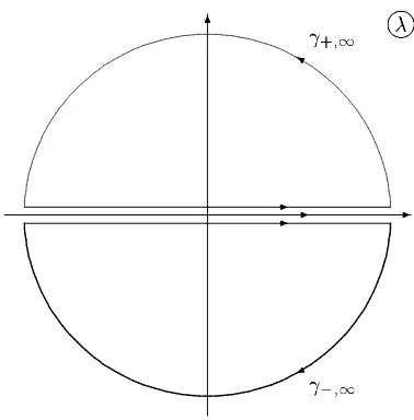
Figure 1. The contoursγ±=R∪γ±∞.
3.2 The Riemann–Hilbert problem
The equations (3.4) and (3.5) can be written down as
X+(x, λ) =X−(x, λ)G(x, λ), λ∈R, (3.7)
where
G(x, λ) = e−iλJ xG0(λ)eiλJ x.
Likewise the second pair of FAS satisfy
˜
X+(x, λ) = ˜X−(x, λ) ˜G(x, λ), λ∈R (3.8)
with
˜
G(x, λ) = e−iλJ xG˜0(λ)eiλJ x G˜0(λ) =
11 +ρ−ρ+ ρ− ρ+ 11
.
Equation (3.7) (resp. equation (3.8)) combined with (3.6) is known in the literature [24] as a Riemann–Hilbert problem (RHP) with canonical normalization. It is well known that RHP with canonical normalization has unique regular solution; the matrix-valued solutionsX0+(x, λ) and X0−(x, λ) of (3.7), (3.6) is called regular if detX0±(x, λ) does not vanish for anyλ∈C±.
Let us now apply the contour-integration method to derive the integral decompositions of X±(x, λ). To this end we consider the contour integrals
J1(λ) = 1 2πi
I
γ+
dµ µ−λX
+(x, µ)− 1
2πi I
γ− dµ µ−λX
−(x, µ),
and
J2(λ) = 1 2πi
I
γ+
dµ µ−λX˜
+(x, µ)− 1
2πi I
γ− dµ µ−λX˜
−(x, µ),
Each of these integrals can be evaluated by Cauchy residue theorem. The result forλ∈C+
are
J1(λ) =X+(x, λ) +
N
X
j=1
Res
µ=λ+j
X+(x, µ)
µ−λ +
N
X
j=1
Res
µ=λ−j
X−(x, µ)
µ−λ , (3.9)
J2(λ) = ˜X+(x, λ) +
N
X
j=1
Res
µ=λ+j
˜
X+(x, µ)
µ−λ +
N
X
j=1
Res
µ=λ−j
˜
X−(x, µ)
µ−λ . (3.10)
The discrete sums in the right hand sides of equations (3.9) and (3.10) naturally provide the contribution from the discrete spectrum of L. For the sake of simplicity we assume that L has a finite number of simple eigenvalues λ±j ∈ C±; for additional details see [10]. Let us clarify
the above statement. For the 2×2 Zakharov–Shabat problem it is well known that the discrete eigenvalues of L are provided by the zeroes of the transmission coefficients a±(λ), which in that case are scalar functions. For the more general 2r×2r Zakharov–Shabat system (1.1) the situation becomes more complex because now a±(λ) are r×r matrices. The discrete eigenval-ues λ±j now are the points at which a±(λ) become degenerate and their inverse develop pole singularities. More precisely, we assume that in the vicinities of λ±j a±(λ), c±(λ) and their inverse ˆa±(λ), ˆc±(λ) have the following decompositions in Laurent series
a±(λ) =a±j + (λ−λ±j) ˙a±j +· · ·, c±(λ) =c±j + (λ−λ±j) ˙c±j +· · ·,
ˆ
a±(λ) = aˆ ±
j
λ−λ±j + ˆ˙a ±
j +· · ·, ˆc±(λ) =
ˆ c±j λ−λ±j + ˆ˙a
±
j +· · · ,
where all the leading coefficients a±j , ˆa±j c±j , ˆc±j are degenerate matrices such that
ˆ
a±ja±j =a±j aˆ±j = 0, ˆc±j c±j =c±j ˆc±j = 0.
In addition we have more relations such as
ˆ
a±ja˙±j + ˆ˙a±j a±j =11, ˆc±j c˙±j + ˆ˙c±j c±j =11,
that are needed to ensure that the identities ˆa±(λ)a±(λ) = 11, ˆc±(λ)c±(λ) = 11 etc hold true for all values ofλ.
The assumption that the eigenvalues are simple here means that we have considered only first order pole singularities of ˆa±j(λ) and ˆc±j(λ). After some additional considerations we find that the ‘halfs’ of the Jost solutions|ψ±(x, λ)iand |φ±(x, λ)isatisfy the following relationships forλ=λ±j
|ψj±(x)ˆc±j i=±|φ±j (x)τj±i, |φ±j (x)ˆa±j i=±|ψ±j (x)ρ±j i,
where
|ψj±(x)i=|ψ±(x, λ±j)i, |φ±j (x)i=|φ±(x, λ±j)i, ρ±j = ˆc±j dj±=b±j aˆ±j , τj±= ˆa±j bj±=d±j ˆc±j
These considerations allow us to calculate explicitly the residues in equations (3.9), (3.10)
where |0istands for a collection ofr columns whose components are all equal to 0.
We can also evaluateJ1(λ) andJ2(λ) by integrating along the contours. In integrating along the infinite semi-circles of γ±,∞ we use the asymptotic behavior of X±(x, λ) and ˜X±(x, λ) for
Equations (3.13), (3.14) can be viewed as a set of singular integral equations which are equivalent to the RHP. For the MNLS these were first derived in [25].
We end this section by a brief explanation of how the potential Q(x, t) can be recovered provided we have solved the RHP and know the solutionsX±(x, λ). First we take into account that X±(x, λ) satisfy the differential equation
idX ±
dx +Q(x, t)X
±(x, λ)−λ[J, X±(x, λ)] = 0 (3.15)
which must hold true for all λ. From equation (3.6) and also from the integral equations (3.13), (3.14) one concludes thatX±(x, λ) and their inverse ˆX±(x, λ) are regular for λ→ ∞and allow
Inserting these into equation (3.15) and taking the limit λ→ ∞ we get
Q(x, t) = lim
λ→∞λ(J−X
±(x, λ)JXˆ±(x, λ)]) = [J, X
4
The generalized Fourier transforms
It is well known that the ISM can be interpreted as a generalized Fourier [10] transform which maps the potentialQ(x, t) onto the minimal sets of scattering dataTi. Here we briefly formulate these results and in the next Section we will analyze how they are modified under the reduction conditions.
The generalized exponentials are the ‘squared solutions’ which are determined by the FAS and the Cartan–Weyl basis of the corresponding algebra as follows
Ψ±α =χ±(x, λ)Eαχˆ±(x, λ), Φ±α =χ±(x, λ)E−αχˆ±(x, λ), α∈∆+1.
4.1 Expansion over the ‘squared solutions’
The ‘squared solutions’ are complete set of functions in the phase space [10]. This allows one to expand any function over the ‘squared solutions’.
Let us introduce the sets of ‘squared solutions’
{Ψ}={Ψ}c∪ {Ψ}d, {Φ}={Φ}c∪ {Φ}d, {Ψ}c≡Ψ+α(x, λ), Ψ−−α(x, λ), i < r, λ∈R ,
{Ψ}d ≡
n
Ψ+α;j(x), Ψ˙+α;j(x), Ψ−−α;j(x), Ψ˙−−α;j(x)oN
j=1, {Φ}c≡Φ+−α(x, λ), Φ−α(x, λ), i < r, λ∈R ,
{Φ}d≡
n
Φ−+α;j(x), Φ˙+−α;j(x), Φ−α;j(x), Φ˙−α;j(x)oN
j=1,
where the subscripts ‘c’ and ‘d’ refer to the continuous and discrete spectrum ofL. The ‘squared solutions’ in bold-face Ψ+α, . . . are obtained from Ψ+α, . . . by applying the projector P0J, i.e.
Ψ+α(x, λ) =P0JΨ+α(x, λ).
Using the Wronskian relations one can derive the expansions over the ‘squared solutions’ of two important functions. Skipping the calculational details we formulate the results [10]. The expansion of Q(x) over the systems{Φ±}and {Ψ±}takes the form
Q(x) = i
π
Z ∞
−∞
dλ X
α∈∆+1
τα+(λ)Φ+α(x, λ)−τα−(λ)Φ−−α(x, λ)
+ 2
N
X
k=1
X
α∈∆+1
τα+;jΦ+α;j(x) +τα−;jΦ−−α;j(x), (4.1)
Q(x) =−i
π
Z ∞
−∞
dλ X
α∈∆+1
ρ+α(λ)Ψ+−α(x, λ)−ρ−α(λ)Ψ−α(x, λ)
−2
N
X
k=1
X
α∈∆+1
ρ+α;jΨ+−α;j(x) +ρ−α;jΨ−α;j(x). (4.2)
The next expansion is of ad−J1δQ(x) over the systems{Φ±}and {Ψ±}
ad−J1δQ(x) = i 2π
Z ∞
−∞
dλ X
α∈∆+1
δτα+(λ)Φ+α(x, λ) +δτ−
α(λ)Φ−−α(x, λ)
+
N
X
k=1
X
α∈∆+1
ad−J1δQ(x) = i 2π
Z ∞
−∞
dλ X
α∈∆+1
δρ+α(λ)Ψ+−α(x, λ) +δρ−α(λ)Ψ−α(x, λ)
+
N
X
k=1
X
α∈∆+1
δW˜−+α;j(x)−δW˜α−;j(x), (4.4)
where
δW±±α;j(x) =δλ±j τα±;jΦ˙±±α;j(x) +δτα±;jΦ±±α;j(x), δW˜∓±α;j(x) =δλ±j ρ±α;jΨ˙±∓α;j(x) +δρ±α;jΨ±∓α;j(x)
and Φ±±α;j(x) =Φ±±α(x, λ±j), ˙Φ
±
±α;j(x) =∂λΦ±±α(x, λ)|λ=λ±j.
The expansions (4.1), (4.2) is another way to establish the one-to-one correspondence bet-ween Q(x) and each of the minimal sets of scattering data T1 and T2 (4.6). Likewise the expansions (4.3), (4.4) establish the one-to-one correspondence between the variation of the potentialδQ(x) and the variations of the scattering data δT1 andδT2.
The expansions (4.3), (4.4) have a special particular case when one considers the class of variations of Q(x, t) due to the evolution int. Then
δQ(x, t)≡Q(x, t+δt)−Q(x, t) = ∂Q
∂t δt+ (O)((δt)
2).
Assuming thatδtis small and keeping only the first order terms inδtwe get the expansions for ad−J1Qt. They are obtained from (4.3), (4.4) by replacing δρ±α(λ) andδτα±(λ) by ∂tρ±α(λ) and
∂tρ±α(λ).
4.2 The generating operators
To complete the analogy between the standard Fourier transform and the expansions over the ‘squared solutions’ we need the analogs of the operator D0 =−id/dx. The operatorD0 is the
one for which eiλx is an eigenfunction: D0eiλx=λeiλx. Therefore it is natural to introduce the
generating operators Λ± through
(Λ+−λ)Ψ+−α(x, λ) = 0, (Λ+−λ)Ψ−α(x, λ) = 0, (Λ+−λ±j )Ψ+∓α;j(x) = 0,
(Λ−−λ)Φ+α(x, λ) = 0, (Λ−−λ)Φ−−α(x, λ) = 0, (Λ+−λ±j )Φ+±α;j(x) = 0,
where the generating operators Λ± are given by
Λ±X(x)≡ad−J1
idX
dx + i
Q(x),
Z x
±∞
dy[Q(y), X(y)]
. (4.5)
The rest of the squared solutions are not eigenfunctions of neither Λ+ nor Λ−
(Λ+−λ+j ) ˙Ψ
+
−α;j(x) =Ψ+−α;j(x), (Λ+−λ
−
j ) ˙Ψ
−
α;j(x) =Ψ−α;j(x),
(Λ−−λ+j ) ˙Φ
+
ir;j(x) =Φ+α;j(x), (Λ−−λ
−
j ) ˙Φ
−
α;j(x) =Φ−α;j(x),
i.e., ˙Ψ+α;j(x) and ˙Φ
+
α;j(x) are adjoint eigenfunctions of Λ+ and Λ−. This means that λ±j , j =
1, . . . , N are also the discrete eigenvalues of Λ± but the corresponding eigenspaces of Λ± have double the dimensions of the ones of L; now they are spanned by bothΨ±∓α;j(x) and ˙Ψ±∓α;j(x).
4.3 The minimal sets of scattering data
Obviously, given the potential Q(x) one can solve the integral equations for the Jost solutions which determine them uniquely. The Jost solutions in turn determine uniquely the scattering matrix T(λ) and its inverse ˆT(λ). But Q(x) contains r(r −1) independent complex-valued functions of x. Thus it is natural to expect that at most r(r −1) of the coefficients in T(λ) for λ ∈ R will be independent; the rest must be functions of those. The set of independent
coefficients of T(λ) are known as the minimal set of scattering data.
The completeness relation for the ‘squared solutions’ ensure that there is one-to-one corre-spondence between the potential Q(x, t) and its expansion coefficients. Thus we may use as minimal sets of scattering data the following two sets Ti ≡Ti,c∪Ti,d
(simple) discrete eigenvalues of L and ρ±j and τj± characterize the norming constants of the corresponding Jost solutions.
Remark 2. A consequence of equation (2.11) is the fact that S±(λ),T±(λ) ∈SO(2r). These factors can be written also in the form
S±(λ) = exp
An important consequence of the expansions is the theorem [10]
Theorem 1. Any nonlinear evolution equation (NLEE) integrable via the inverse scattering method applied to the Lax operator L (1.1) can be written in the form
i ad−J1∂Q
∂t + 2f(Λ)Q(x, t) = 0, (4.8)
where the function f(λ) is known as the dispersion law of this NLEE. The generic MMKdV equation is a member of this class and is obtained by choosing f(λ) = −4λ3. If Q(x, t) is
a solution to (4.8) then the corresponding scattering matrix satisfy the linear evolution equation
idT
or equivalently and therefore can be considered as generating functionals of integrals of motion for the NLEE.
Let us, before going into the non-trivial reductions, briefly discuss the Hamiltonian formula-tions for the generic (i.e., non-reduced) MMKdV type equaformula-tions. It is well known (see [10] and the numerous references therein) that the class of these equations is generated by the so-called recursion operator Λ = 1/2(Λ++ Λ−) which is defined by equation (4.5).
If no additional reduction is imposed one can write each of the equations in (4.8) in Hamil-tonian form. The corresponding HamilHamil-tonian and symplectic form for the MMKV equation are given by
The Hamiltonian can be identified as proportional to the fourth coefficientI4 in the asymptotic
expansion of A+(λ) (5.15) over the negative powers ofλ
This series of integrals of motion is known as the principal one. The first three of these integrals take the form
We will remind also another important result, namely that the gradient of Ik is expressed
through Λ as
∇QT(x)Ik=−
1 2Λ
k−1Q(x, t).
Then the Hamiltonian equations written through Ω(0) and the Hamiltonian vector field XH(0)
in the form
Ω(0)(·, XH(0)) +δH(0)= 0 (4.11)
forH(0) given by (4.10) coincides with the MMKdV equation.
Then the Hamiltonian equations of motions
dqij
dt ={qij, H
(0)} (0),
dpij
dt ={pij, H
(0)}
(0) (4.12)
with the above choice for H(0) again give the MMKdV equation.
Along with this standard Hamiltonian formulation there exist a whole hierarchy of them. This is a special property of the integrable NLEE. The hierarchy is generated again by the recursion operator and has the form
HMMKdV(m) =−8I4+m, Ω(m)=
1 i
Z ∞
−∞ dxtr
ad−J1δQ(x)∧′ J,Λmad−J1δQ(x)
.
Of course there is also a hierarchy of Poisson brackets
{F, G}(m)= i
Z ∞
−∞
dxtr∇QT(x)F, h
J,Λ−m∇QT(x)G i
.
For a fixed value of m the Poisson bracket {·,·}(m) is dual to the symplectic form Ω(m) in the
sense that combined with a given Hamiltonian they produce the same equations of motion. Note that since Λ is an integro-differential operator in general it is not easy to evaluate explicitly its negative powers. Using this duality one can avoid the necessity to evaluate negative powers of Λ.
Then the analogs of (4.11) and (4.12) take the form:
Ω(m)(·, XH(m)) +δH(m)= 0, (4.13)
dqij
dt ={qij, H
(−m)} (m),
dpij
dt ={pij, H
(−m)}
(m), (4.14)
where the hierarchy of Hamiltonians is given by:
H(m) =−4X
k
fkIk+1−m. (4.15)
The equations (4.13) and (4.14) with the Hamiltonian H(m) given by (4.15) will produce the
NLEE (4.8) with dispersion lawf(λ) =Pkfkλk for any value of m.
Remark 3. It is a separate issue to prove that the hierarchies of symplectic structures and Poisson brackets have all the necessary properties. This is done using the spectral decompositions of the recursion operators Λ±which are known also as the expansions over the ‘squared solutions’ of L. We refer the reader to the review papers [26, 10] where he/she can find the proof of the completeness relation for the ‘squared solutions’ along with the proof that any two of the symplectic forms introduced above are compatible.
4.4 The reduction group of Mikhailov
The reduction group GR is a finite group which preserves the Lax representation (1.1), i.e. it
ensures that the reduction constraints are automatically compatible with the evolution. GRmust
have two realizations: i) GR ⊂Autg and ii) GR ⊂ ConfC, i.e. as conformal mappings of the
complexλ-plane. To eachgk ∈GRwe relate a reduction condition for the Lax pair as follows [5]
Ck(L(Γk(λ))) =ηkL(λ), Ck(M(Γk(λ))) =ηkM(λ), (4.16)
where Ck∈Autg and Γk(λ)∈ConfCare the images ofgk and ηk= 1 or −1 depending on the
choice of Ck. Since GR is a finite group then for each gk there exist an integer Nk such that
gNk
More specifically the automorphisms Ck, k = 1, . . . ,4 listed above lead to the following
reductions for the potentialsU(x, t, λ) and V(x, t, λ) of the Lax pair
U(x, t, λ) =Q(x, t)−λJ, V(x, t, λ) =
2
X
k=0
λkVk(x, t)−4λ3J,
of the Lax representation
1) C1(U†(κ1(λ))) =U(λ), C1(V†(κ1(λ))) =V(λ), (4.17)
2) C2(UT(κ2(λ))) =−U(λ), C2(VT(κ2(λ))) =−V(λ), (4.18)
3) C3(U∗(κ1(λ))) =−U(λ), C3(V∗(κ1(λ))) =−V(λ), (4.19)
4) C4(U(κ2(λ))) =U(λ), C4(V(κ2(λ))) =V(λ), (4.20)
where
a) κ1(λ) =λ∗, b) κ2(λ) =−λ.
The condition (4.16) is obviously compatible with the group action.
5
Finite order reductions of MMKdV equations
In order that the potential Q(x, t) be relevant for a DIII type symmetric space it must be of the form
Q(x, t) = X
α∈∆+1
(qα(x, t)Eα+pα(x, t)E−α),
or, equivalently
Q(x, t) = X
1≤i<j≤r
qij(x, t)Eei+ej+pij(x, t)E−ei−ej
. (5.1)
In the next two subsections we display new reductions of the MMKdV equations.
5.1 Class A Reductions preserving J
The class A reductions can be applied also to the MMKdV type equations. The corresponding automorphisms C preserve J, i.e.C−1JC =J and are of the form
C−1U†(x, λ∗)C =U(x, λ), U(x, λ) =Q(x, t)−λJ,
where J is an element of the Cartan subalgebra dual to the vector e1+e2 +e3 +e4. In the
typical representation of so(8)U(x, λ) takes the form
U(x, t, λ) =
λ11 q(x, t)
p(x, t) −λ11
, q(x, t) =
q14 q13 q12 0
q24 q23 0 q12
q34 0 q23 −q13
0 q34 −q24 q14
,
p(x, t) =
p14 p24 p34 0
p13 p23 0 p34
p12 0 p23 −p24
0 p12 −p13 p14
Remark 4. The automorphisms that satisfyC−1JC =J naturally preserve the eigensubspaces
of adJ; in other words their action on the root space maps the subsets of roots ∆±1 onto
themselves: C∆±1 = ∆±1.
We list here several inequivalent reductions of the Zakharov–Shabat system. In the first one we chooseC =C0 to be an element of the Cartan subgroup
C0 = exp πi 4
X
k=1
skhk
!
,
where sk take the values 0 and 1. This condition means that C02 = 11, so this will be a Z2
-reduction, or involution. Then the first example of Z2-reduction is
C0−1Q†(x, t)C0 =Q(x, t),
or in components
pij =ǫijqij∗, ǫij =ǫiǫj, ǫj =eπisj =±1.
Obviously ǫj takes values±1 depending on whether sj equals 0 or 1.
The next examples ofZ2-reduction correspond to several choices ofCas elements of the Weyl
group eventually combined with the Cartan subgroup elementC0
C1 =Se1−e2Se3−e4C0,
where Sei−ej is the Weyl reflection related to the root ei−ej. Again we have a Z2-reduction,
or an involution
C1−1Q†(x, t)C1 =Q(x, t).
Written in components it takes the form (ǫ12=ǫ34= 1)
p12=−q∗12, p24=−ǫ23q∗13, p23=−ǫ13q∗14,
p14=−ǫ13q∗23, p13=−ǫ23q∗24, p34=−q∗34.
The corresponding Hamiltonian and symplectic form take the form
8I3=−
Z ∞
−∞
∂xq∗12∂xq12+∂xq34∗ ∂xq34+ǫ13(q23∗ ∂xq14+∂xq∗14∂xq23)
+ǫ23 ∂xq24∗ ∂xq13+∂xq13∗ ∂xq24)
dx+ Z ∞
−∞
ǫ12q12∗ q12+q∗34q34
+ǫ13(q∗23q14+q24∗ q13) +ǫ23(q∗14q23+q13∗ q24)
2
dx
+ Z ∞
−∞
|q13q24+q12q34−q14q23|2dx,
Ω(0) = 1 i
Z ∞
−∞
δq12∗ ∧δq12+ǫ13(q23∗ ∧δq14+δq∗14∧δq23)
+ǫ23(δq∗24∧δq13+δq13∗ ∧δq24) +δq34∗ ∧δq34
dx.
Another inequivalent examples ofZ2-reduction corresponds to
The involution is C2−1Q†(x, t)C
2 =Q(x, t), or in components it takes the form
p12=−ǫ12q∗12, p24=−ǫ13q∗14, p23=−ǫ14q13∗ ,
p14=−ǫ23q∗24, p13=−ǫ24q∗23, p34=−ǫ34q34∗ .
As a consequence we get
8I3=−
Z ∞
−∞
ǫ12∂xq∗12∂xq12+ǫ34∂xq∗34∂xq34+ǫ14∂xq13∗ ∂xq23
+ǫ23∂xq∗24∂xq14+ǫ24∂xq∗23∂xq13+ǫ13∂xq14∗ ∂xq24
dx
+ Z ∞
−∞
ǫ12|q12|2+ǫ34|q34|2+ǫ23q24∗ q14+ǫ24q∗23q13+ǫ14q∗13q23+ǫ13q14∗ q24
2
dx
+ǫ12ǫ34
Z ∞
−∞
|q13q24+q12q34−q14q23|2dx,
Ω(0) = 1 i
Z ∞
−∞
ǫ12δq12∗ ∧δq12+ǫ34q34∗ ∧δq34+ǫ23δq∗24∧δq14
+ǫ14δq∗13∧δq23+ǫ24δq23∗ ∧δq13+ǫ13δq∗14∧δq24
dx.
Next we consider aZ3-reduction generated by C3 =Se
1−e2Se2−e3 which also maps J intoJ.
It splits each of the sets ∆±1 into two orbits which are
(O)±1 ={±(e1+e2) ±(e2+e3) ±(e1+e3)},
(O)±2 ={±(e1+e4) ±(e2+e4) ±(e3+e4)}.
In order to be more efficient we make use of the following basis ing(0)
E(αk)=
2
X
p=0
ω−kpC3−kEαC3k, Fα(k) =
2
X
p=0
ω−kpC3−kFαC3k,
where ω= exp(2πi/3) and α takes values e1+e2 and e1+e4. Obviously
C3−1E(αk)C3 =ωkE(αk), C3−1F(αk)C3 =ωkFα(k). (5.2)
In addition, since ω∗ = ω−1 we get (E(0)α )† =F(0)α and (E(αk))† =Fα(3−k) for k = 1,2. Then we
introduce the potential
Q(x, t) =
3
X
k=0
X
α
qα(k)(x, t)E(αk)+p(αk)(x, t)F(αk).
In view of equation (5.2) the reduction condition (4.17) leads to the following relations between the coefficients
p(0)12 = (q(0)12)∗, p(12k)=ωk(q12(3−k))∗, q(12k)=ωk(p(312−k))∗,
p(0)14 = (q(0)14)∗, p(14k)=ωk(q14(3−k))∗, q(14k)=ωk(p(314−k))∗, (5.3)
where k = 1,2. It is easy to check that from the conditions (5.3) there follows p12(k) = q12(k) =
Similarly the reduction (4.18) leads to
q12(0) =−(q12(0))∗, q(12k)=−ω3−k(q12(3−k))∗, q(14k)=−ω3−k(q(314−k))∗,
p(0)12 =−(p(0)12)∗, p(12k)=−ω3−k(p12(3−k))∗, p(14k)=−ω3−k(p(314−k))∗, (5.4)
where k= 1,2. Again from the conditions (5.4) there follows p(12k) =q12(k) =p(14k) =q(14k) = 0. So we are left with two pairs of purely imaginary independent functions: q(0)12,q14(0) and p(0)12,q(0)14.
The corresponding Hamiltonian and symplectic form are obtained from the slightly more general formulae below by imposing the constraints (5.3) and (5.4). Here for simplicity we skip the upper zeroes in qij and pij
HMMKdV=
1 6
Z ∞
−∞
dx ∂x2q12∂xp12−∂xq12∂x2p12+∂x2q14∂xp14−∂xq14∂x2p14
− 1
12 Z ∞
−∞
p212q122 ∂x−p212∂xq212+q142 ∂xp214−p212∂xq212
dx,
8I3=
4 3
Z ∞
−∞
dx(∂xq12∂xp12+∂xq14∂xp14)−
8 9
Z ∞
−∞
q214p214+q122 p212dx,
Ω(0) = 4 3
Z ∞
−∞
dx (δq14∧δp14+δq12∧δp12),
i.e. in this case we get two decoupled mKdV equations. The Z4-reduction generated by C4 =Se
1−e2Se2−e3Se3−e4 also maps J into J. It splits each
of the sets ∆±1 into two orbits which are
(O)±1 ={±(e1+e2)±(e2+e3)±(e3+e4)±(e1+e4)},
(O)±2 ={±(e1+e3)±(e2+e4)}.
Again we make use of a convenient basis in g(0)
E(αk)=
3
X
p=0
i−kpC4−kEαC4k, F(αk) =
3
X
p=0
i−kpC4−kFαC4k,
where α takes valuese1+e2 and e1+e3. Obviously
C4−1E(αk)C4 =ikE(αk), C4−1Fα(k)C4 =ikF(αk) (5.5)
and in addition, (E(0)α )† = Fα(0), (Eα(k))† =Fα(4−k) and (E(αk))∗ =Eα(4−k) for k= 1,2,3. Then we
introduce the potential
Q(x, t) =
3
X
k=0
X
α
qα(k)(x, t)E(αk)+p(αk)(x, t)F(αk).
In view of equation (5.5) the reduction condition (4.17) leads to the following relations between the coefficients
p(0)α = (q(0)α )∗, p(αk)=ik(qα(4−k))∗, q(αk)=ik(p(4α−k))∗ (5.6)
fork= 1,2,3. Herepα,qαcoincide withp12,q12(resp.p13,q13) forα=e1+e2(resp.α=e1+e3).
Analogously the reduction (4.18) gives
for k = 1,2,3. Both conditions (5.6), (5.7) lead to p(12k) = q12(k) = p(14k) = q14(k) = 0 for k = 1,3. In addition it comes up that E(0)13 = E(2)13 = F13(0) = F13(2). So we are left with only two pairs of independent functionsp(0)12,q(0)12 andp(2)12,q(2)12. We provide below slightly more general formulae for the corresponding Hamiltonian and symplectic form which are obtained by imposing the constraints (5.6) or (5.7); again for simplicity of notations we skip the upper zeroes in qij(0)
and p(0)ij and replaceqij(2) and p(2)ij by ˜qij and ˜pij
∂tq2∨+∂x3q2∨+
3 2(q
∨
2p∨2 −q0∨p∨0)∂xq∨2 +
3 2(q
∨
2p∨0 +q0∨p∨2)∂xq∨0 = 0,
∂tp∨0 +∂x3p∨0 +
3 2(q
∨
2p∨0 −q∨0p∨2)∂xp∨0 +
3 2(−q
∨
0p∨0 +q2∨p∨2)∂xp∨2 = 0,
∂tp∨2 +∂x3p∨2 +
3 2(q
∨
2p∨2 −q∨0p∨0)∂xp∨0 +
3 2(q
∨
0p∨2 −q2∨p∨0)∂xp∨2 = 0.
5.2 Class B Reductions mapping J into −J
The class B reductions of the Zakharov–Shabat system change the sign ofJ, i.e.C−1JC =−J; therefore we must have also λ→ −λ.
Remark 5. Note that adJ has three eigensubspaces Wa, a = 0,±1 corresponding to the
eigenvalues 0 and ±2. The automorphisms that satisfy C−1JC = −J naturally preserve the
eigensubspace W0 but map W−1 onto W1 and vice versa. In other words their action on the root space maps the subset of roots ∆+1 onto ∆−1 and vice versa: C∆±1 = ∆∓1.
Here we first consider
C5 =Se1−e2Se1+e2Se3−e4Se3+e4C0.
Obviously the product of the the above 4 Weyl reflections will change the sign of J. Its effect on Qin components reads
qij =−ǫijq∗ij, pij =−ǫijp∗ij, ǫij =ǫiǫj,
i.e. some of the components of Qbecome purely imaginary, others may become real depending on the choice of the signs ǫj.
There is no Z3 reduction for the so(8) MMKdV that maps J into −J. So we go directly
to the Z4-reduction generated by C6 =Se
1+e2Se2+e3Se3+e4 which mapsJ into −J. The orbits
of C3 are
(O)±1 ={±(e1+e2)∓(e2+e3)±(e3+e4)∓(e1+e4)},
(O)±2 ={±(e1+e3)∓(e2+e4)}.
Again we make use of a convenient basis in g(0)
E(αk)=
3
X
p=0
i−kpC6−kEαC6k, F(αk)=
3
X
p=0
i−kpC6−kFαC6k,
where α takes valuese1+e2 and e1+e3. Obviously
C6−1E(αk)C6 = ikE(αk), C6−1Fα(k)C6 = ikF(αk), (5.9)
where again (E(0)α )† = F(0)α , (Eα(k))† = Fα(4−k) and (E(αk))∗ = Eα(4−k) for k = 1,2,3. Then we
introduce the potential
Q(x, t) =
3
X
k=0
X
α
qα(k)(x, t)E(αk)+p(αk)(x, t)F(αk).
In view of equation (5.9) the reduction condition (4.17) leads to the following relations between the coefficients
while the reduction (4.18) gives below slightly more general formulae for the corresponding Hamiltonian and symplectic form which are obtained by imposing the constraints (5.10) or (5.11) and again for simplicity we skip the upper zeroes in qij and pij and replace q(2)12 and p(2)12 by ˜q12 and ˜p12
Now we get two specially coupled mKdV-type equations.
The class B reductions also render all the symplectic forms and Hamiltonians in the hierarchy real-valued. They allow to render the corresponding systems of MMKdV equations into ones involving only real-valued fields. ‘Half’ of the Hamiltonian structures do not survive these reductions and become degenerate. This holds true for all symplectic forms Ω(2m)and integrals
of motion I2m with even indices. However the other ‘half’ of the hierarchy with Ω(2m+1) and
integrals of motionI2m+1 remains and provides Hamiltonian properties of the MMKdV.
Now we get four specially coupled mKdV-type equations given by
Obviously in the system (5.12) we can put both q0,q2 real with the result
The class B reductions also render all the symplectic forms and Hamiltonians in the hierarchy real-valued. They allow to render the corresponding systems of MMKdV equations into ones involving only real-valued fields. ‘Half’ of the Hamiltonian structures do not survive these reductions and become degenerate. This holds true for all symplectic forms Ω(2m)and integrals
of motion I2m with even indices. However the other ‘half’ of the hierarchy with Ω(2m+1) and
integrals of motionI2m+1 remains and provides Hamiltonian properties of the MMKdV.
5.3 Ef fects of class A reductions on the scattering data
The reflection coefficientsρ±(λ) andτ±(λ) are defined only on the realλ-axis, while the diagonal blocks a±(λ) and c±(λ) (or, equivalently, D±(λ)) allow analytic extensions for λ∈C
±. From the equations (2.9) there follows that
a+(λ)c−(λ) = (11 +ρ−ρ+(λ))−1, a−(λ)c+(λ) = (11 +ρ+ρ−(λ))−1, (5.13) c−(λ)a+(λ) = (11 +τ+τ−(λ))−1, c+(λ)a−(λ) = (11 +τ−τ+(λ))−1. (5.14)
Given T1 (resp. T2) we determine the right hand sides of (5.13) (resp. (5.14)) for λ ∈ R.
Combined with the facts about the limits
lim
each of the relations (5.13), (5.14) can be viewed as a RHP with canonical normalization. Such RHP can be solved explicitly in the one-component case (provided we know the locations of their zeroes) by using the Plemelj–Sokhotsky formulae [24]. These zeroes are in fact the discrete eigenvalues of L. One possibility to make use of these facts is to take log of the determinants of both sides of (5.13) getting
where A(λ) =A+(λ) for λ∈ C+ and A(λ) =−C−(λ) for λ∈C
−. In deriving (5.16) we have also assumed that λ±j are simple zeroes of A±(λ) and C±(λ).
Let us consider a reduction condition (4.17) with C1 from the Cartan subgroup: C1 =
diag (B+, B−) where the diagonal matricesB±are such thatB2±=11. Then we get the following constraints on the sets T1,2
ρ−(λ) = (B−ρ+(λ)B+)†, ρ−j = (B−ρ+jB+)†, λ−j = (λ+j )∗,
τ−(λ) = (B+τ+(λ)B−)†, τj−= (B+τj+B−)
†, λ−
j = (λ
+
j )
∗,
where j= 1, . . . , N. For more details see Subsections4.3 and 4.4.
Remark 6. For certain reductions such as, e.g. Q = −Q† the generalized Zakharov–Shabat system L(λ)ψ = 0 can be written down as an eigenvalue problem Lψ = λψ(x, λ) where L
is a self-adjoint operator. The continuous spectrum of L fills up the whole real λ-axis thus ‘leaving no space’ for discrete eigenvalues. Such Lax operators have no discrete spectrum and the corresponding MNLS or MMKdV equations do not have soliton solutions.
From the general theory of RHP [24] one may conclude that (5.13), (5.14) allow unique solu-tions provided the number and types of the zeroesλ±j are properly chosen. Thus we can outline a procedure which allows one to reconstruct not only T(λ) and ˆT(λ) and the corresponding potentialQ(x) from each of the setsTi,i= 1,2:
i) Given T2 (resp. T1) solve the RHP (5.13) (resp. (5.14)) and construct a±(λ) and c±(λ) for
λ∈C±.
ii) Given T1 we determineb±(λ) and d±(λ) as
b±(λ) =ρ±(λ)a±(λ), d±(λ) =c±(λ)ρ±(λ),
or ifT2 is known then
b±(λ) =a±(λ)τ±(λ), d±(λ) =τ±(λ)c±(λ).
iii) The potential Q(x) can be recovered from T1 by solving the RHP (3.7) and using equa-tion (3.16).
Another method for reconstructingQ(x) fromTj uses the interpretation of the ISM as gene-ralized Fourier transform, see [27,28,29].
Let in this subsection all automorphismsCi are of class A. Therefore acting on the root space
they preserve the vector
r
P
k=1
ekwhich is dual toJ, and as a consequence, the corresponding Weyl
group elements map the subset of roots ∆+1 onto itself.
Remark 7. An important consequence of this is thatCi will map block-upper-triangular (resp.
block-lower-triangular) matrices like in equation (3.2) into matrices with the same block struc-ture. The block-diagonal matrices will be mapped again into block-diagonal ones.
From the reduction conditions (4.17)–(4.20) one gets, in the limit x→ ∞that
a) C1((κ1(λ)J)†) =λJ, b) C2((κ2(λ)J)T) =−λJ,
c) C3((κ3(λ)J)∗) =λJ, d) C4((κ4(λ)J)) =λJ. (5.17)
Using equation (5.17) andCi(J) =J one finds that:
It remains to take into account that the reductions (4.17)–(4.20) for the potentials of Llead to the following constraints on the scattering matrix T(λ)
a) C1(T†(λ∗)) = ˆT(λ), b) C2(TT(−λ)) = ˆT(λ),
c) C3((T∗(−λ∗)) =T(λ), d) C4(T(λ)) =T(λ).
These results along with Remark 7 lead to the following results for the generalized Gauss factors ofT(λ)
a) C1(S+,†(λ∗)) = ˆS−(λ), C1(T−,†(λ∗)) = ˆT+(λ),
b) C2(S+,T(−λ)) = ˆS−(λ), C2(T−,T(−λ)) = ˆT+(λ),
c) C3(S±,∗(−λ∗)) =S±(λ), C3(T±,∗(−λ∗)) =T±(λ),
d) C4(S±(λ)) =S±(λ), C4(T±(λ)) =T±(λ)
and
a) C1(D+,†(λ∗)) = ˆD−(λ), b) C2(D+,T(−λ)) = ˆD−(λ),
c) C3(D±,∗(−λ)) =D±(λ), d) C4(D±(λ)) =D±(λ).
5.4 Ef fects of class B reductions on the scattering data
In this subsection all automorphisms Ci are of class B. Therefore acting on the root space they
map the vector
r
P
k=1
ek dual toJ into− r
P
k=1
ek. As a consequence, the corresponding Weyl group
elements map the subset of roots ∆+1 onto ∆−1 ≡ −∆+1.
Remark 8. An important consequence of this is that Ci will map block-upper-triangular into
block-lower-triangular matrices like in equation (3.2) and vice versa. The block-diagonal matrices will be mapped again into block-diagonal ones.
Now equation (5.17) withCi(J) =−J leads to
a) κ1(λ) =−λ∗, b) κ2(λ) =λ, c) κ3(λ) =λ∗, d) κ4(λ) =−λ.
The reductions (4.17)–(4.20) for the potentials of L lead to the following constraints on the scattering matrix T(λ):
a) C1(T†(−λ∗)) = ˆT(λ), b) C2(TT(λ)) = ˆT(λ),
c) C3((T∗(λ∗)) =T(λ), d) C4(T(−λ)) =T(λ).
Then along with Remark 8 we find the following results for the generalized Gauss factors of T(λ)
a) C1(S±,†(−λ∗)) = ˆS±(λ), C1(T±,†(−λ∗)) = ˆT±(λ),
b) C2(S±,T(λ)) = ˆS±(λ), C2(T±,T(λ)) = ˆT±(λ),
c) C3(S+,∗(λ∗)) =S−(λ), C3(T−,∗(λ∗)) =T+(λ),
d) C4(S+(−λ)) =S−(λ), C4(T−(−λ)) =T+(λ)
and
a) C1(D±,†(−λ∗)) = ˆD±(λ), b) C2(D±,T(λ)) = ˆD±(λ),
6
The classical
r
-matrix and the NLEE of MMKdV type
One of the definitions of the classical r-matrix is based on the Lax representation for the cor-responding NLEE. We will start from this definition, but before to state it will introduce the following notation
n
U(x, λ)⊗
′ U(y, µ)
o
,
which is an abbreviated record for the Poisson bracket between all matrix elements of U(x, λ) and U(y, µ)
n
U(x, λ)⊗
′ U(y, µ)
o
ik,lm ={Uik(x, λ), Ulm(y, µ)}.
In particular, if U(x, λ) is of the form
U(x, λ) =Q(x, t)−λJ, Q(x, t) =X
i<r
(qirEir+priEri),
and the matrix elements of Q(x, t) satisfy canonical Poisson brackets
{qks, pri}= iδikδrsδ(x−y),
then n
U(x, λ)⊗
′ U(y, µ)
o
= iX
i<r
(Eir⊗Eri−Eri⊗Eir)δ(x−y).
The classicalr-matrix can be defined through the relation [19] n
U(x, λ)⊗
′ U(y, µ)
o
= i [r(λ−µ), U(x, λ)⊗11 +11⊗U(y, µ)]δ(x−y), (6.1)
which can be understood as a system of N2 equation for the N2 matrix elements of r(λ−µ). However, these relations must hold identically with respect toλandµ, i.e., (6.1) is an overdeter-mined system of algebraic equations for the matrix elements ofr. It is far from obvious whether such r(λ−µ) exists, still less obvious is that it depends only on the difference λ−µ. In other words far from any choice for U(x, λ) and for the Poisson brackets between its matrix elements allow r-matrix description. Our system (6.1) allows an r-matrix given by
r(λ−µ) =−1
2
P
λ−µ, (6.2)
where P is a constantN2×N2 matrix
P =
N
X
α∈∆+
(Eα⊗E−α+E−α⊗Eα) + r
X
k=1
hk⊗hk.
The matrixP possesses the following special properties
[P, X⊗11 +11⊗X] = 0 ∀X ∈g.
By using these properties ofP we are getting
i.e., the r.h.s. of (6.1) does not contain Q(x, t). Besides:
[P, λJ⊗11 +µ11⊗J] = (λ−µ) [P, J⊗11]
=−2(λ−µ)
X
α∈∆+1
(Eα⊗E−α−E−α⊗Eα)
, (6.4)
where we used the commutation relations between the elements of the Cartan–Weyl basis. The comparison between (6.3), (6.4) and (6.1) leads us to the result, that r(λ−µ) (6.2) indeed satisfies the definition (6.1).
Remark 9. It is easy to prove that equation (6.1) is invariant under the reduction condi-tions (4.17) and (4.18) of class A, so the corresponding reduced equations have the same r -matrix. However (6.1) is not invariant under the class B reductions and the corresponding reduced NLEE do not allow classicalr-matrix defined through equation (6.1).
Let us now show, that the classicalr-matrix is a very effective tool for calculating the Poisson brackets between the matrix elements of T(λ). It will be more convenient here to consider periodic boundary conditions on the interval [−L, L], i.e.Q(x−L) = Q(x+L) and to use the fundamental solution T(x, y, λ) defined by
idT(x, y, λ)
dx +U(x, λ)T(x, y, λ) = 0, T(x, x, λ) =11.
Skipping the details we just formulate the following relation for the Poisson brackets between the matrix elements of T(x, y, λ) [19]
n
T(x, y, λ)⊗
′ T(x, y, µ)
o
= [r(λ−µ), T(x, y, λ)⊗T(x, y, µ)]. (6.5)
The corresponding monodromy matrix TL(λ) describes the transition from −L to L and
TL(λ) =T(−L, L, λ). The Poisson brackets between the matrix elements ofTL(λ) follow directly
from equation (6.5) and are given by n
TL(λ)⊗
′ TL(µ)
o
= [r(λ−µ), TL(λ)⊗TL(µ)].
An elementary consequence of this result is the involutivity of the integrals of motion IL,k
from the principal series which are from the expansions of
ln deta+L(λ) = ∞
X
k=1
IL,kλ−k, −ln detc−L(λ) =
∞
X
k=1
IL,kλ−k,
ln detc+L(λ) = ∞
X
k=1
JL,kλ−k, −ln deta−L(λ) =
∞
X
k=1
JL,kλ−k. (6.6)
An important property of the integralsIL,k andJL,k is their locality, i.e. their densities depend
only on Qand its x-derivatives.
The simplest consequence of the relation (6.5) is the involutivity ofIL,k,JL,k. Indeed, taking
the trace of both sides of (6.5) shows that {trTL(λ),trTL(µ)}= 0. We can also multiply both
sides of (6.5) by C⊗C and then take the trace using equation (6.3); this proves
In particular, for C=11 +J and C =11−J we get the involutivity of
tra+L(λ),tra+L(µ) = 0, tra−L(λ),tra−L(µ) = 0,
trc+L(λ),trc+L(µ) = 0, trc−L(λ),trc−L(µ) = 0.
Equation (6.5) was derived for the typical representation V(1) of G ≃SO(2r), but it holds true also for any other finite-dimensional representation of G. Let us denote by V(k)≃ ∧kV(1)
the k-th fundamental representation of G; then the element TL(λ) will be represented in V(k)
by∧kT
L(λ) – thek-th wedge power ofTL(λ), see [12]. In particular, if we consider equation (6.5)
in the representationV(n)and sandwich it between the highest and lowest weight vectors inV(n)
we get [30]
{deta+L(λ),deta+L(µ)}= 0, {detc−L(λ),detc−L(µ)}= 0. (6.7)
Likewise considering (6.5) in the representation V(m) and sandwich it between the highest
and lowest weight vectors in V(m) we get
{deta−L(λ),deta−L(µ)}= 0, {detc+L(λ),detc+L(µ)}= 0. (6.8)
Since equations (6.7) and (6.8) hold true for all values of λ and µ we can insert into them the expansions (6.6) with the result
{IL,k, IL,p}= 0, {JL,k, JL,p}= 0, k, p= 1,2, . . . .
Somewhat more general analysis along this lines allows one to see that only the eigenvalues of a±L(λ) andc±L(λ) produce integrals of motion in involution.
Taking the limit L→ ∞ we are able to transfer these results also for the case of potentials with zero boundary conditions. Indeed, let us multiply (6.5) byE(y, λ)⊗E(y, µ) on the right and by E−1(x, λ)⊗E−1(x, µ) on the left, where E(x, λ) = exp(−iλJx) and take the limit for
x→ ∞,y → −∞. Since
lim
x→±∞
eix(λ−µ)
λ−µ =±iπδ(λ−µ),
we get n
T(λ)⊗
′ T(µ)
o
=r+(λ−µ)T(λ)⊗T(µ)−T(λ)⊗T(µ)r−(λ−µ),
r±(λ−µ) =− 1 2(λ−µ)
r
X
k=1
hk⊗hk+
X
α∈∆+0
(Eα⊗E−α+E−α⊗Eα)
±iπδ(λ−µ)Π0J,
where Π0J is defined by
Π0J =
X
α∈∆+1
(Eα⊗E−α−E−α⊗Eα).
Analogously we prove that i) the integrals Ik = lim
L→∞IL,k and Jp = limL→∞JL,p are in involution, i.e.
{Ik, Ip}={Ik, Jp}={Jk, Jp}= 0,