El e c t ro n ic
Jo ur
n a l o
f P
r o
b a b il i t y
Vol. 15 (2010), Paper no. 61, pages 1893–1929. Journal URL
http://www.math.washington.edu/~ejpecp/
The maximum of Brownian motion with parabolic drift
∗
Svante Janson
Department of Mathematics Uppsala University
PO Box 480
SE-751 06 Uppsala, Sweden [email protected] http://www.math.uu.se/~svante/
Guy Louchard
Département d’Informatique Université Libre de Bruxelles CP 212, Boulevard du Triomphe
B-1050 Bruxelles Belgium [email protected]
Anders Martin-Löf
Department of Mathematics Stockholm University
SE-10691 Stockholm
Sweden
Abstract
We study the maximum of a Brownian motion with a parabolic drift; this is a random variable that often occurs as a limit of the maximum of discrete processes whose expectations have a maximum at an interior point. We give new series expansions and integral formulas for the distribution and the first two moments, together with numerical values to high precision.
Key words:Brownian motion, parabolic drift, Airy functions. AMS 2000 Subject Classification:Primary 60J65.
Submitted to EJP on February 2, 2010, final version accepted October 28, 2010.
∗A major part of this research was done while the authors all visited Institut Mittag-Leffler, Djursholm, Sweden, during
1
Introduction
LetW(t)be a two-sided Brownian motion withW(0) =0; i.e.,(W(t))t≥0 and(W(−t))t≥0 are two independent standard Brownian motions. We are interested in the process
Wγ(t):=W(t)−γt2 (1.1)
for a givenγ >0, and in particular in its maximum
Mγ:= max
−∞<t<∞Wγ(t) =−∞max<t<∞ W(t)−γt
2. (1.2)
We also consider the corresponding one-sided maximum
Nγ:= max
0≤t<∞Wγ(t) =0max≤t<∞ W(t)−γt
2. (1.3)
Since the restrictions of W to the positive and negative half-axes are independent, we have the relation
Mγ
d
=max(Nγ,Nγ′) (1.4)
whereNγ′is an independent copy ofNγ.
Note that (a.s.) Wγ(t)→ −∞ as t → ±∞, so the maxima in (1.2) and (1.3) exist and are finite; moreover, they are attained at unique points and Mγ,Nγ >0. It is easily seen (e.g., by Cameron– Martin) thatMγandNγ have absolutely continuous distributions.
1.1
Scaling
For anya>0,W(at)=d a1/2W(t)(as processes on(−∞,∞)), and thus
Mγ= max
−∞<t<∞ W(at)−γ(at)
2
d = max
−∞<t<∞ a
1/2W(t)
−a2γt2=a1/2Ma3/2γ, (1.5)
and similarly
Nγ
d
=a1/2Na3/2γ. (1.6)
The parameterγis thus just a scale parameter, and it suffices to consider a single choice ofγ. We choose the normalizationγ=1/2 as the standard case, and writeM:=M1/2,N:=N1/2. In general, (1.5)–(1.6) witha= (2γ)−2/3yield
Mγ= (d 2γ)−1/3M, Nγ= (d 2γ)−1/3N. (1.7)
Remark 1.1. More generally, if a,b>0, then
max
−∞<t<∞ aW(t)−bt
2=aM
b/a
d =
a4
2b
1/3
The distributions ofNandM were characterized by Groeneboom[10, Theorem 3.1 – Corollary 3.2]; see also Daniels and Skyrme[8]. ([8]gives also formulas for the meanEM.) The descriptions there
are, however, rather complicated. The purpose of this paper is to provide further, more explicit, formulas for the distribution function of M and, in particular, for its moments; our formulas are either integrals or series, and invariably involve the Airy function Ai. We also provide companion result forN. (Our results are based on Groeneboom[10]and the related results by Salminen[21].) Other simple integral formulas for the distribution and density functions of N and M have been given by Groeneboom[11]; these are not obviously equivalent to our formulas. It seems likely that there may be further similar formulas that have not yet been discovered, possibly including some even simpler ones. In particular, it would be interesting to find simple integral formulas for higher moments ofM.
The main results are given in Section 2, with proofs and further details in Sections 3–5. We illustrate the use of the formulas by using them to compute the density and the first two moments ofM and N numerically; we discuss the numerical computations in Section 6.
We use many more or less well-known results for Airy functions; for convenience we have collected them in Appendices A–B. Finally, Appendix C discusses an interesting integral equation, while Ap-pendix D contains an alternative proof of an important formula used in our proofs.
1.2
Background
The random variableM is studied by Barbour[4], Daniels and Skyrme[8]and Groeneboom[10]. (Further results on N are given by Lachal[16].) M arises as a natural limit distribution in many different problems, and in many related problems its expectationEM enters in a second order term
for the asymptotics of means or in improved normal approximations. For various examples and general results, see for example Daniels[6; 7], Daniels and Skyrme[8], Barbour[4; 5], Smith[22], Louchard, Kenyon and Schott [19], Steinsaltz [23], Janson[15]. As discussed in several of these papers, the appearance of M in these limit results can be explained as follows, ignoring technical conditions: Consider the maximum over time t of a random processXn(t), defined on a compact interval I, for example [0, 1], such that as n→ ∞, the mean EXn(t), after scaling, converges to
deterministic function f(t), and that the fluctuations Xn(t)−EXn(t) are of smaller order and,
after a different scaling, converge to a gaussian process G(t). If we assume that f is continuous on I and has a unique maximum at a point t0 ∈ I, then the maximum of the process Xn(t) is
attained close to t0. Assuming that t0 is an interior point of I and that f is twice differentiable at t0 with f′′(t0) 6= 0, we can locally at t0 approximate f by a parabola and G(t)−G(t0) by a two-sided Brownian motion (with some scaling), and thus maxtXn(t)−Xn(t0) is approximated by a scaling constant times the variable M, see Barbour [4]. In the typical case where the mean of Xn(t) is of order n and the Gaussian fluctuations are of order n1/2, it is easily seen that the correct scaling is that n−1/3(maxtXn(t)−Xn(t0)) −→d c M, for some c > 0, which for the mean gives EmaxtXn(t) = n f(t0) +n1/3cEM +o(n1/3), see [4; 6; 7]. As examples of applications in
algorithmic and data structures analysis, this type of asymptotics appears in the analysis of linear lists, priority queues and dictionaries[18; 19]and in a sorting algorithm[15].
Remark 1.2. The locationof the maximum in (1.2) is also of interest in various applications, see Groeneboom and Wellner[12]. It has been studied by several authors; in particular, Groeneboom
analytical and numerical formulas. (Groeneboom[10]describes even the joint distribution of the maximum M and its location, see also Daniels and Skyrme [8].) The location of the maximum is not considered in the present paper.
2
Main results
The mean of M can be expressed as integrals involving the Airy functions Ai and Bi, for example as follows. (For general definitions and properties of Airy functions, see [1, Section 10.4]. We remind the reader that Ai(t)and Bi(t)are linearly independent solutions of f′′(t) =t f(t), and that Ai(t)→0 as t→+∞.)
Theorem 2.1(Daniels and Skyrme[8]).
EM=−2
−1/3
2πi
Z i∞
−i∞
zdz Ai(z)2 =
2−1/3 2πi
Z ∞
−∞
ydy
Ai(i y)2 (2.1)
=22/3
Z ∞
0
Ai(t)2+p3Ai(t)Bi(t)
Ai(t)2+Bi(t)2 dt (2.2)
=22/3Re
1+ip3
Z ∞
0
Ai(t) Ai(t) +iBi(t) dt
(2.3)
= 2 2/3
π
Z ∞
0
p
3Bi(t)2−p3Ai(t)2+2Ai(t)Bi(t)
Ai(t)2+Bi(t)22 tdt. (2.4)
The expressions (2.1) and (2.2) (unfortunately with typos in the latter) are given by Daniels and Skyrme[8]. Since detailed proofs of the formulas are not given there, we for completeness give a complete proof in Section 5. (The proof includes a direct analytical verification of the equivalence of (2.1) and (2.2), which was left open in[8].)
By (A.1) and (A.8), |Ai(i y)| increases superexponentially as y → ±∞, while Ai(t) decreases su-perexponentially and Bi(t) increases superexponentially as t → ∞; hence, the integrands in the integrals in Theorem 2.1 all decrease superexponentially and the integrals converge rapidly, so they are suited for numerical calculations. We obtain by numerical integration (usingMaple), improving the numerical values in[4; 5; 8; 7],
EM=0.99619 30199 28363 11660 37766 . . . (2.5)
We do not know any similar integral formulas for the second moment of M (or higher moments). Instead we give expressions using infinite series, summing over the zerosak,k≥1, of the Airy func-tion, see Appendix A. Recall that these zeros all are real and negative, so we have 0>a1>a2>. . . , see[1, (10.4.94)]and Appendix A; note that|ak| ≍k2/3, see (A.30). (We use xn≍ yn, for two se-quences of positive numbersxn and yn, to denote that 0<lim infn→∞xn/yn≤lim supn→∞xn/yn<
∞; this is also denotedxn= Θ(yn).)
We first introduce more notation. LetFN(x)be the distribution function ofN, i.e.,FN(x):=P(N ≤
x), and letFM(x)be the distribution function ofM; further, letGN(x) =1−FN(x) =P(N>x)and
GM(x) =1−FM(x) =P(M> x)be the corresponding tail probabilities. Then, by (1.4),
and, equivalently,
GM(x):=1−(1−GN(x))2=2GN(x)−GN(x)2. (2.7)
If we knowGN(x), we thus know the distribution of bothN andM, and we can compute moments
by
ENp=p
Z ∞
0
xp−1GN(x)dx, (2.8)
EMp=p
Z ∞
0
xp−1GM(x)dx=p
Z ∞
0
xp−1 2GN(x)−GN(x)2
dx. (2.9)
Two formulas for the distribution function are given in the following theorem. Others are given in (3.3) and Lemma 3.5. The proof is given in Section 3. Hi is the function defined in (A.16).
Theorem 2.2. The distribution functions of M and N are FM(x) = (1−GN(x))2 and FN(x) =1−
GN(x), where
GN(x) =π
∞ X
k=1 Hi(ak)
Ai′(ak)Ai(ak+2
1/3x), x >0. (2.10)
The sum converges conditionally but not absolutely for every x > 0. Alternatively, with an absolutely convergent sum, for x≥0,
GN(x) = Ai(2 1/3x)
Ai(0) +
∞ X
k=1
πHi(ak) +a−k1
Ai′(ak) Ai(ak+2
1/3x). (2.11)
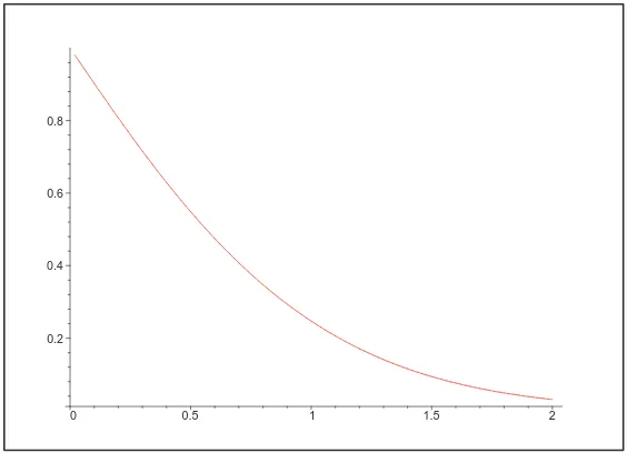
The functionGN(x)is plotted in Figure 1.
Remark 2.3. By (A.4) and (A.30), for any fixed x > 0, |Ai(ak+21/3x)| is usually of the order
|ak|−1/4 ≍k−1/6, and using also (A.31) and (A.33), the summands in (2.10) are (typically) of the
order k−1/6−1/6−2/3 = k−1, so this sum is not absolutely convergent. (For some values of k, the term may be smaller thank−1because ak+21/3x may be close to another zero, but such cases are infrequent and do not prevent the series from being absolutely divergent.)
On the other hand, by (A.22),πHi(z) +z−1=O(|z|−4)on the negative real axis, and it follows that the terms in (2.11) areO(k−3), so the series is absolutely convergent. Moreover, since Ai is bounded on the real axis (see (A.1) and (A.4)), the sum in (2.11) converges uniformly for x ≥ 0, and is thus a continuous function of x; this is no surprise since we already have remarked that N has an absolutely continuous distribution, soG is continuous. Note also that (2.11) forx =0 is the trivial GN(0) =1, since each Ai(ak) =0, while (2.10) does not hold for x=0.
The sum in (2.11) can be differentiated termwise and we have the following result, proved in Section 3.
Theorem 2.4. N and M have absolutely continuous distributions with infinitely differentiable density functions, for x>0,
fN(x) =−21/3Ai
′(21/3x) Ai(0) −2
1/3
∞ X
k=1
πHi(ak) +a−k1 Ai′(ak) Ai
′(a
k+21/3x), (2.12)
0.2 0.4 0.6 0.8
0 0.5 1 1.5 2
Figure 1: GN(x)
0.2 0.4 0.6 0.8
0 0.5 1 1.5 2
0.1 0.2 0.3 0.4 0.5 0.6 0.7
0 0.5 1 1.5 2
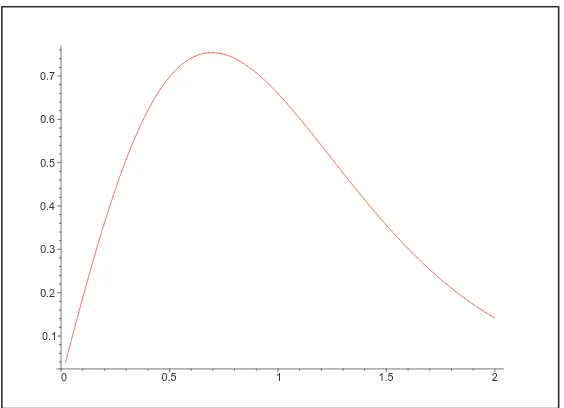
Figure 3: fM(x)
Integral formulas for fN(x) will be given in (3.10) and (5.10). The density functions fN(x) and
fM(x)are plotted in Figures 2 and 3.
Remark 2.5. In contrast, the sum
21/3π
∞ X
k=1 Hi(ak) Ai′(ak)Ai
′(a
k+21/3x) (2.14)
obtained by termwise differentiation of (2.10) isnot convergent for any x ≥ 0, as will be seen in Section 3.
Moments of M and N now can be obtained from (2.8) and (2.9) by integrating (2.11) termwise. This yields the following result; see Section 4 for proofs as well as related integral formulas. For higher moments, see Remark 4.4.
We define for convenience
ϕ(k):=πHi(ak) +a−k1. (2.15)
By (A.22),ϕ(k) =O(|ak|−4) =O(k−8/3). Recall also the function Gi(z) =Bi(z)−Hi(z), see (A.17). Theorem 2.6. The means and second moments of M and N are given by the absolutely convergent sums
EN= 1
21/33Ai(0)− π 21/3
∞ X
k=1
= 1
The numerical value forEM agrees with the one in (2.5).
Further formulas for moments are given in Theorems 4.5 and 4.6.
3
Distributions
Salminen[21, Example 3.2]studied the hitting time
τ:=inf{t≥0 : x+W(t) =−βt2}, (3.1)
for the density function ofτ. Note thatτis a defective random variable, and thatτ=∞if and only if mint≥0(x+W(t) +βt2)>0. By symmetry,W =d −W, and thus
P(τ=∞) =P max
t≥0(W(t)−βt 2
Hence, choosingβ=1/2,
If we formally integrate termwise we obtain (2.10), from (A.16). However, as seen in Remark 2.3, the sum is not absolutely convergent, so we cannot use e.g. Fubini’s theorem, and we have to justify the termwise integration by a more complicated argument.
Remark 3.1. We have |ak| = Θ(k2/3) by (A.30), and |Ai′(ak)| = Θ(k1/6) by (A.31); further, for
fixed x > 0, Ai(ak+21/3x) = O(|ak|−1/4) = O(k−1/6) by (A.4). Hence the sums in (3.2) and (3.3) converge rapidly for each fixed t, because of the negative termakt in the exponent. But the convergence rate is small for smallt, and when integrating we have the problem just described. We begin by converting the sum in (3.2) into a residue integral. Fix θ0 ∈ (0,π/2) and x0 ∈ around the N first zeros of Ai; moreover, ΓN does not come too close to any of the zeros; this is made more precise by the estimates in Lemma A.2 and Lemma A.3.
Lemma 3.2. Letτ= τx be the hitting time (3.1)forβ =1/2and some x >0. Then the defective
random variableτhas the density function, for t>0,
fτ(t) = thus the integrand in (3.4),Φ(z)say, is bounded by
Φ(z) =O exp −2−1/3t|Rez| −t3/6=O exp −2−1/3t|Rez|. This shows both thatRΓΦ(z)dzis absolutely convergent, and that
Z
Φ(z)has simple poles at the zeros ak of Ai, and evaluating
R ΓN
Φ(z)dz by residues, we see that it equals the partial sum of theN first terms of (3.2). Consequently, (3.2) yieldsRΓ
N
Remark 3.3. The contourΓin (3.4) can be deformed to the imaginary axis, using the estimate in Lemma A.1. Hence, settingz=21/3si,
et3/6fτ(t) = 1 2π
Z ∞
−∞
eistAi(2
1/3(si+x))
Ai(21/3si) ds. (3.6)
Moreover, this holds also for t ≤0, with fτ(t) =0, since the right-hand side of (3.6) then easily is shown to vanish: writing it again as a line integral along the imaginary axis we can move the line of integration to Rez=σ, for anyσ >a1, and fort≥0 we may letσ→+∞, again using Lemma A.1. This exhibits et3/6fτ(t) as the inverse Fourier transform of s 7→ Ai(21/3(si +x))/Ai(21/3si). By Lemma A.1, this function is integrable and in L2, and using (A.1) and (A.2), it is seen that so is its derivative, which implies that the Fourier transformet3/6fτ(t)is integrable. The Fourier inversion formula yields Z
∞
−∞
et3/6fτ(t)e−istdt= Ai(2
1/3(si+x))
Ai(21/3si) , −∞<s<∞, (3.7) and, more generally, by analytic continuation,
Z ∞
−∞
et3/6fτ(t)e−z tdt =
Ai(21/3(z+x))
Ai(21/3z) , Rez≥0 (3.8)
(and, in fact, for Rez>a1). This formula for the Laplace transform is (in a more general version) given by Groeneboom [10, Theorem 2.1], where et3/6fτ(t) is denoted h1/2,x(t); see also (5.5) below. Conversely, this formula from[10]yields by Fourier inversion (3.6) and (3.4), so we could have used it instead of (3.2) from[21]as our starting point. We give an alternative proof of (3.8) in Appendix D, which thus gives us a self-contained proof of Lemma 3.2. (Groeneboom[10], Salminen
[21]and our Appendix D use similar methods. See also Appendix C for another approach.)
Remark 3.4. For our purposes we consider only x >0 in (3.1). For x <0, the hitting time is a.s. finite; its distribution is found in Martin-Löf[20].
Lemma 3.5. For x>0,
GN(x) = 1 2i
Z
Γ
Hi(z)Ai(z+21/3x)
Ai(z) dz. (3.9)
Proof. We haveGN(x) =P(τ <∞) =R∞
0 fτ(t)dt. Now integrate (3.4) with respect to t and inter-change the order of integration, which is allowed by Fubini’s theorem and the estimate Lemma A.1, which implies that forz∈Γ, the integrand in (3.4) is bounded byO exp(−c x|z|1/2−t3/6). The result follows by (A.16) (and a change of variablest=21/3t1).
The integral in (3.9) is absolutely convergent and converges rapidly for any fixed x > 0 by Lemma A.1 and (A.21). We denote the integrand in (3.9) byΨ(z) = Ψ(z;x).
Proof of Theorem 2.2. Fix x > 0. By (A.21) and Lemmas A.1 and A.2, for z = RNei(ϕ+π) with
|ϕ| ≤ π2, Ψ(z) = O |z|−1exp −x|z|1/2|ϕ|/π. It follows that RΓ
NΨ(z)dz−
R
ΓΨ(z)dz → 0 as
N→ ∞, and thusGN(z) = 1
2ilimN→∞
R
ΓNΨ(z)dz. Evaluating
R
To obtain (2.11), we take out the first term in the expansion (A.20) of Hi(z), and write (3.9) as
GN(x) = 1 2i
Z
Γ
(Hi(z) +π−1z−1)Ai(z+21/3x)
Ai(z) dz−
1 2iπ
Z
Γ
Ai(z+21/3x) zAi(z) dz.
The first integral can be converted to a sum of residues by the argument just given for (3.9), which yields the sum in (2.11). Indeed, we have better estimates now, and the resulting sum is absolutely convergent as seen in Remark 2.3.
For the second integral we instead close the contour on the right, by a large circular arc{Rei t}fort fromπ−θ0 to−(π−θ0); it follows by Lemma A.1 that the error tends to 0 asR→ ∞. Inside this closed contour, Ai has no zeros, so the only pole is atz =0 where the residue is Ai(21/3x)/Ai(0). The result follows, noting that we go around this contour in the negative direction.
Remark 3.6. We may also use the expansion (A.20) of Hi with more terms. In general, subtracting the sum with L terms in (A.20) from Hi in (3.9) yields an integral that can be converted to a sum of residues as above; this sum is similar to the ones in (2.10) and (2.11), and the terms are now of orderk−1−2L. We also have the integral with the subtracted terms; this is a linear combination of terms of the type RΓz−n−1Ai(z+21/3x)/Ai(z), which as above equals −2πi times the residue at 0, so this integral can be written as a combination of derivatives of Ai at 21/3x and 0; by the equation Ai′′(z) = zAi(z), and successive derivations of this equation, the result can be written as p1(x)Ai(21/3x) +p2(x)Ai′(21/3x) for some polynomials p1 and p2 (depending on L), whose coefficients are rational functions in Ai(0)and Ai′(0). We leave the details to the reader.
Proof of Theorem 2.4. If|argz|< π−δand|z| ≥1, say, then by Lemma A.3,|Ai′(z)/Ai(z)| ≍ |z|1/2. More generally, using also Ai′′(z) =zAi(z), and differentiating this equation further, by induction, Ai(m)(z)/Ai(z) =O(|z|m/2)for every fixedm≥0.
It follows by Lemma A.1 and (A.21) that for every fixedm≥0, x in a fixed interval(x0,x1) with 0<x0<x1, andz∈Γ,
∂m
∂xmΨ(z;x) =O
|z|−1|z+x|m/2e−c x|z|1/2
=O
|z|m/2−1e−c x0|z|1/2
.
Consequently, we can differentiate (3.9) under the integral sign an arbitrary number of times; this shows thatGis infinitely differentiable on(0,∞)and thatN has an infinitely differentiable density
fN =−G′given by
fN(x) =−G′(x) = 2 1/3i
2
Z
Γ
Hi(z)Ai′(z+21/3x)
Ai(z) dz. (3.10)
This integral can be evaluated as a sum of residues as for (2.11) in the proof of Theorem 2.2 above, by first addingπ−1z−1 to Hi(z), which yields (2.12). Alternatively, and perhaps simpler, (A.5) and (A.31) imply that, uniformly for 0≤ x ≤ x0 for any fixed x0 >0, Ai′(ak+21/3x) =O(|ak|1/4) =
O(Ai′(ak)), and thus the terms in the sum in (2.12) areO(|πHi(ak) +ak−1|) =O(|ak|−4) =O(k−8/3). Hence we can integrate the sum in (2.12) termwise; equivalently, we can differentiate (2.11) termwise, which yields (2.12).
To see that the sum (2.14) does not converge for any x >0, let y := 21/3x. Take x =|ak| − y in (A.5). Since then, by Taylor’s formula and (A.30),
2
3(|ak| −y) 3/2= 2
3|ak| 3/2
−y|ak|1/2+o(1) =
π(4k−1)
4 − y(3πk/2)
1/3+o(1),
we obtain
Ai′(ak+y) =−π−1/2|ak|1/4 cos(πk−y(3πk/2)1/3+o(1)) +o(1) and thus
Ai′(ak+y) Ai′(ak) =
cos(πk− y(3πk/2)1/3) +o(1)
cos(πk) +o(1) =cos(y(3πk/2)
1/3) +o(1).
Let In be the interval [c(2πn)3,c(2πn+ 1)3], with c := 2y−3/(3π). For k ∈ In, we have
y(3πk/2)1/3 ∈ [2πn, 2πn+1] and thus Ai′(a
k+ y)/Ai′(ak) ≥ cos 1+o(1) > 0.5, if n is large.
Further, by (A.19) and (A.30), Hi(ak) ∼ π−1|ak|−1 ∼ π−1(3π/2)−2/3k−2/3. Hence the term in (2.14),tksay, satifies, for some constantsc1,c2>0 andk∈In,
tk≥c1k−2/3≥c2n−2.
Since there areΘ(n2)integers inIn, the sum over them isΘ(1), and thus the sum in (2.14) diverges. (The casex =0 is simple.)
4
Moments
Lemma 4.1. For every fixed p≥1, uniformly in a≥0,
Z ∞
0
xp−1|Ai(x−a)|dx=O(ap−1/4+1), (4.1)
Z ∞
0
xp−1|Ai(x−a)|2dx=O(ap−1/2+1). (4.2)
Proof. For 0≤x <awe havexp−1≤ap−1and|Ai(x−a)|=O((a−x)−1/4)by (A.4), so
Z a
0
xp−1|Ai(x−a)|dx =O
ap−1
Z a
0
(a−x)−1/4dx
=O ap−1a3/4,
and similarlyRa 0 x
p−1
|Ai(x−a)|2dx=O ap−1a1/2. For largerx we use the rapid decrease in (A.1), which implies
Z ∞
a
xp−1|Ai(x−a)|dx=
Z ∞
0
(y+a)p−1|Ai(y)|dy=O(1+ap−1),
Proof of Theorem 2.6. Write (2.11) as
where we for convenience definea0=0 and
= 2
and (2.18) follows by the definition ofϕ(k).
Similarly, (4.3) converges absolutely in L1((0,∞),xdx) and L2((0,∞),xdx) too, and termwise integration in (4.3) yields, using (B.15), (A.26), (B.6), (B.25), (B.19), (B.21),
Z ∞
2xdx, and (2.21) follows. The numerical evaluation is done byMaple, using the method discussed in Section 6.
Remark 4.2. The formula above for R0∞GN(x)2dx may be simplified. In fact, (Ai′(0)/Ai(0))2 =
P∞
k=1a− 2
k by (B.27), and thus the formula can be written
Z ∞
This can be seen as an instance of Parseval’s formula, see Remark B.1. However, although simpler than our expression above, this sum converges more slowly and is less suitable for our purposes.
Remark 4.3. As is well-known, see[1, 10.4.4–5], Ai(0) =3−2/3/Γ(2/3) =3−1/6Γ(1/3)/(2π)and Ai′(0) =−3−1/3/Γ(1/3) =−31/6Γ(2/3)/(2π). We prefer to keep Ai(0)and Ai′(0)in our formulas.
with more terms taken out of the expansion (A.20) of Hi, as discussed in Remark 3.6. We do not pursue the details.
We can also give integral formulas based on Lemma 3.5.
Theorem 4.5. The moments of M and N are given by, for any real p>0,
ENp=−p2−p/3−1i
Z
Γ
Z ∞
0
xp−1Ai(z+x)dx Hi(z) Ai(z)dz,
EMp=−p2−p/3i Z
Γ
Z ∞
0
xp−1Ai(z+x)dx Hi(z) Ai(z)dz
+p2−p/3−2
Z
Γ Z
Γ
Z ∞
0
xp−1Ai(z+x)Ai(w+x)dx Hi(z) Ai(z)
Hi(w) Ai(w)dzdw.
Proof. Immediate from (2.8)–(2.9) and Lemma 3.5 (with a change of variables x →2−1/3x). The double and triple integrals converge absolutely by Lemma A.1 and (A.21).
For integerp, the integrals over x in Theorem 4.5 can be evaluated by the formulas in Appendix B. In particular, by (B.1) and (B.22),
EM=−2−1/3i Z
Γ
AI(z)Hi(z) Ai(z) dz
+2−7/3
Z
Γ Z
Γ
Ai(z)Ai′(w)−Ai′(z)Ai(w) z−w
Hi(z)Hi(w)
Ai(z)Ai(w) dzdw. (4.6) Although there is no singularity whenz=win the double integral in (4.6), it may be advantageous to use different, disjoint, contours for z and w. Remember that Γ = Γ(θ0,x0). We choose θ1 ∈ (θ0,π/2) and x1 ∈(x0, 0), and let Γ′:= Γ(θ1,x1). Then ΓandΓ′ are disjoint; moreover, ifz ∈Γ andw∈Γ′, then
|z−w| ≥cmax(|z|,|w|) (4.7)
for somec>0. Furthermore, (4.7) holds also ifz∈Γn andw∈Γ′M with M≥2N. We can replace the double integralsRΓRΓin Theorem 4.5 and (4.6) byRΓRΓ′. Taking residues, this leads to another formula with sums over Airy zeros.
Theorem 4.6.
EN=2−1/3π2 ∞ X
k=1
Hi(ak)(Hi(ak)−Bi(ak)), (4.8)
EM =2−1/3π2 ∞ X
k=1
Hi(ak)(Hi(ak)−2Bi(ak)). (4.9)
Proof. Let
Q(z,w):=
Z ∞
0
Ai(z+x)Ai(w+x)dx.
The integral converges absolutely by (A.1) for all complexzandw, uniformly in compact sets, and thusQis an entire function of two variables; moreover, (B.5) and (B.9) yield the explicit formulas
Q(z,z) =Ai′(z)2−zAi(z)2, (4.10)
Q(z,w) = Ai(z)Ai
′(w)−Ai′(z)Ai(w)
z−w , z6=w. (4.11)
By Theorem 4.5 and (4.6), usingΓ′as discussed above,
EN=−2−4/3i
First consider the simple integral, R
ΓΦ(z)dz say. It follows from Lemma A.3 and (A.21) that
The sums converge, e.g. by the argument just given, but only the final sum PHi(ak)2 converges absolutely, by (A.32)–(A.34). This yields the result (4.8) forN.
Next consider the double integral. Ifz∈Γandw∈Γ′, orz∈Γn andw∈Γ′m withm≥2n, then by (4.7), (4.11) and Lemma A.3,
, withm=2n, we find that the double integral above equals
By (4.11),Q(aj,ak) =0 when j6=k, andQ(ak,ak) =Ai′(ak)2 by (4.10). Hence the double integral equals−4π2P∞k=1Hi(ak)2.
The result (4.9) follows by combining the terms.
5
Proof of Theorem 2.1
Proof of (2.1). We shall use Groeneboom[10]. Fixγ >0. (We may choose e.g.γ=1/2 as in other parts of this paper by (1.7), but for ease of comparison with[10], and because we find it instructive to see how the homogeneity works, we write the proof for a generalγ.) Fix alsos≥0 and define
Vs:=max
t≥−s(W(t)−γt
2). (5.1)
Thus,V0=Nγ, andVsրV∞=Mγass→ ∞.
For t ≥ −s, the process Ws(t) := W(t)−W(−s) is a Brownian motion, starting at 0 at time −s. Define
e
M=Mes:=max
t≥−s Ws(t)−γt
2=V
s−W(−s), (5.2)
and letτ=τsbe the (a.s. unique) time withWs(τ)−γτ2=Me. Note thatMe ≥W
s(−s)−γs2=−γs2
andτ ≥ −s(strict inequalities hold a.s.) Groeneboom [10, Corollary 3.1] applies to Ws(t)−γt2 (withsreplaced by−sandx =−γs2), and shows thatτandMe have a joint density, fort >−sand
y>x =−γs2,
fτ,Me(t,y) =exp −23γ2(t3+s3) +2γs(y+γs2)hγ,y+γs2(t+s)kγ(t) =exp 43γ2s3+2γs yhγ,y+γs2(t+s)gγ(t).
(5.3)
where the functionshγ,y+γs2, kγ and gγ are given in[10]. Integrating over t ≥ −s we find, with hγ,a(t) =0 fort<0 and ˇgγ(t):= gγ(−t), the density fMe ofMe as, for y>−γs2,
fMe(y) =
Z ∞
−s
f(t,y)dt=exp 4 3γ
2s3+2γs y
Z ∞
−s
hγ,y+γs2(t+s)gγ(t)dt
=exp 43γ2s3+2γs yhγ,y+γs2∗ˇgγ(s). (5.4)
By[10, Theorem 2.1], fora>0,hγ,a ≥0 and hγ,a has the Laplace transform, forλ >0, (see also
Remark 3.3) Z
∞
0
e−λuhγ,a(u)du= Ai (4γ)
1/3a+ξ
Ai(ξ) , ξ:= (2γ
2)−1/3λ. (5.5)
Lettingλց0 we see that
Z ∞
0
hγ,a(u)du=Ai (4γ)1/3a/Ai(0)<∞,
so hγ,a ∈ L1(R) and (5.5) holds for all complex λ with Reλ ≥ 0 by analytic continuation. In
particular,hγ,ahas the Fourier transform, see (3.7),
Ô
hγ,a(ω) =
Z ∞
−∞
e−iωuhγ,a(u)du=
Ai (4γ)1/3a+i(2γ2)−1/3ω
Furthermore, by (5.3), gγ≥0, and by[10, Corollary 3.1], gγ∈L1(R)with the Fourier transform the Fourier inversion formula applies to (5.7), and (5.4) thus yields, for y>−γs2,
fMe(y) =exp 43γ2s3+2γs y2
Multiplying byez y and integrating, we obtain for anyz∈Cthe following, where the double integral
is absolutely convergent by Lemma A.1,
EezMe =
Since Ai is bounded on the negative real axis by (A.4), Lemma B.2 implies that, for Rez>0,
Hence, if Rez≥(4γ)−1/3, say, andv∈R, then, using Cauchy’s integral formula on a large rectangle
In particular, if 2γs>2, say, this holds uniformly for|z|<1, and we may differentiate the analytic functions atz=0 and obtain
EMe = 1
By residue calculus, as with similar integrals in e.g. the proof of Theorem 2.2, this may be written as a sum of residues of 21/3Ai(21/3y+z)/Ai(z)2at the polesak; however, now the poles are double and we omit the details.
Proof of (2.4). The integrand in (2.1) is analytic except at the zeros of Ai, which lie on the negative real axis. Furthermore, by (A.1),|Ai(z)|is exponentially large, so the integrand in (2.1) is exponen-tially small, as|z| → ∞withπ/3+δ≤ |arg(z)| ≤π−δ; in particular whenπ/2≤ |arg(z)| ≤2π/3. Hence, we can deform the integration path from the imaginary axis to any reasonable path in this domain. We choose to integrate along the two rays from the origin with argz=±2π/3, and obtain thus
Proof of (2.2). To prove (2.2), we as above deform the integration path in (2.1) and integrate along the two rays from the origin with argz = ±2π/3 and obtain (5.11). We now use the indefinite
integral Z
and thus, by (5.12) again,
Bi(ze2πi/3)
=0+e2πi/3π The integral along the line frome−2πi/3∞to 0 equals−1 times the complex conjugate of the integral in (5.15), so we obtain from (5.11) and (5.15),
EM =−2
Proof of (2.3). Follows similarly by (5.11) and (5.14), we omit the details.
6
Numerical computation
The sums in Theorem 2.6 converge, but rather slowly. For example, in (2.16), |ϕ(k)Gi(k)| =
|ϕ(k)| |Bi(k)−Hi(k)| ∼ck−17/6 for somec>0, see the asymptotic expansions below.
To obtain numerical values with high accuracy of the sums in (2.16)–(2.21), we therefore use asymp-totic expansions of the summands. More precisely, for each sum, we first computeP199k=1numerically. (All computations are done byMaple.) We then evaluateP∞200 by replacing the summands by the first terms in the following asymptotic expansions. (We provide here only one or two terms in each asymptotic expansions, but we use at least 5 terms in our numerical computations.) We note that Bi(ak)alternates in sign, so for terms containing it, we group the terms withk=2jandk=2j+1 together, for j ≥100. The resulting infinite sums are readily computed numerically. (They can be expressed in the Riemann zeta function at some points.)
S1N:=− π 21/3
∞ X
k=200
ϕ(k)Bi(ak) =− π 21/3
∞ X
j=100
g1(j) =0.5317 . . .·10−8,
S2N:= π 21/3
∞ X
k=200
ϕ(k)Hi(ak) =−0.16722 . . .·10−7,
yieldingE(N) =0.6955289995 . . .. Similarly,EM =S0M+S1M+S2M, with
S0M=0.9961930092 . . . ,
S1M:=− π 21/3
∞ X
k=200
2ϕ(k)Bi(ak) =2S1N=0.10635 . . .·10−7,
S2M:=2−1/3
∞ X
k=200
ϕ(k)2=0.20 . . .·10−13,
yielding EM = 0.9961930199 . . ., which fits with (2.5). Actually, we have 15 digits of precision
with the expansions we have used.
For the second moments, we compute the sums in (2.20) and (2.21) in the same way. For the double sum in (2.21), we compute the sum withk≤199 exactly, and find using asymptotics the tail sum
27/3
∞ X
k=200
k−1
X
j=1
ϕ(k)ϕ(j) (ak−aj)2
=0.4 . . .·10−10.
(We may, for example, use the first term asymptotics forϕ(j)andaj for j≥200, since the sum is small and only a low relative precision is needed.)
The (complementary) distribution functionGN(x)and the density function fN(x)may, for any given
x > 0, be computed to high precision from (2.11) and (2.12) in the same way; for the tails of the sums P∞k=200ϕ(k)Ai(ak+21/3x)/Ai′(ak) and P∞k=200ϕ(k)Ai′(ak+21/3x)/Ai′(ak) we use the asymptotic expansion ofϕ(k)given above together with, see[1, (10.4.94), (10.4.97), (10.4.105)]
and (A.4)–(A.5),
Ai(ak+21/3x)∼(−1)k+1 2 1/6
31/6π2/3sin (3π)
1/3x k1/3k−1/6+. . .
Ai′(ak+21/3x)∼(−1)k+1 3 1/6
21/6π1/3cos (3π)
1/3x k1/3k1/6+. . .
for fixed x, and, as a special case,
Ai′(ak)∼(−1)k+1 3 1/6
21/6π1/3k
1/6+. . .
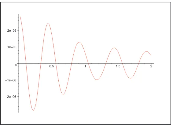
–2e–06 –1e–06 0 1e–06 2e–06
0.5 1 1.5 2
Figure 4: Tail sum fromk=200 for fN(x)
A
Some Airy function estimates
The Airy function Ai(x)and its derivative have along the positive real axis, and more generally as
|z| → ∞with|argz|< π−δfor any fixedδ >0, asymptotic expansions given in full in[1, 10.4.59 and 10.4.61]; we need only the leading terms:
Ai(z)∼ 2p1πz−1/4e−23z 3/2
, (A.1)
Ai′(z)∼ − 1 2pπz
1/4e−23z3/2
. (A.2)
In particular, along the imaginary axis, for y∈R,
|Ai(i y)| ∼ 1 2pπ|y|
−1/4e p
2 3|y|
3/2
. (A.3)
Along the negative real axis, Ai and Ai′oscillate and have zeros; by[1, (10.4.60), (10.4.62)](where further terms are given), we have the asymptotic formulas
Ai(−x) =π−1/2x−1/4 sin 23x3/2+π 4
+o(1)=O(x−1/4), (A.4) Ai′(−x) =−π−1/2x1/4 cos 23x3/2+ π
4
+o(1). (A.5)
and more generally, as|z| → ∞in any domain|argz|< 23π−δ,
Ai(−z) = π−1/2z−1/4
sin
2
3z
3/2 + π 4
1 + O(|z|−3/2) + O |z|−3/2
Ai′(−z) = −π−1/2z1/4
For the companion Airy function Bi(x), we use the following estimate[1, 10.4.63], valid along the positive real axis, and more generally as|z| → ∞with|argz|< π/3−δ,
implicit constants depending on x but not on N orθ),
Proof. By symmetry, it suffices to considerθ =π+ϕ with 0≤ ϕ ≤π/2. Thus z = −RNeiϕ. We
In particular, taking x = 0 we obtain (A.12) for these ϕ. Moreover, comparing (A.15) with the special casex =0, and using (A.14),
Recall also the entire functions Gi and Hi defined by[1, (10.4.44), (10.4.46)]:
Hi(z):=π−1
The integral defining Hi evidently converges for all complexz. There is a similar integral yielding Gi[1, (10.4.42)]:
We have the asymptotics, asx → ∞,[1, (10.4.91)]
Hi(−x)∼π−1x−1. (A.19)
More generally, for Rez<0, expanding exp(−t3/3)in (A.16) yields, for anyL≥0,
Hi(z) =−π−1
L−1
X
ℓ=0 (3ℓ)!
3ℓ z
−3ℓ−1+O
|Rez|−3L−1. (A.20)
In particular, for anyδ >0 and argz∈(π 2 +δ,
3π
2 −δ),
Hi(z) =O|Rez|−1=O|z|−1. (A.21)
More precisely, for suchz,
Hi(z) =−π−1z−1+O|z|−4. (A.22)
We further define, usingR∞
0 Ai(x)dx =1/3[1, 10.4.82],
AI(z):=
Z +∞
z
Ai(t)dt =1 3−
Z z
0
Ai(t)dt; (A.23)
this is well-defined for all complex z and yields an entire function provided the first integral is taken along, for example, a path that eventually follows the positive real axis to +∞. Note that AI′(z) =−Ai(z)and that AI(0) =1/3. Along the real axis we have the limits, by[1, 10.4.82–83],
lim
x→+∞AI(x) =0, (A.24)
lim
x→−∞AI(x) =
Z ∞
−∞
Ai(x)dx =1. (A.25)
In terms of the functions Gi and Hi, we have, see[1, 10.4.47–48],
AI(z) =π Ai(z)Gi′(z)−Ai′(z)Gi(z) (A.26) =1+π Ai′(z)Hi(z)−Ai(z)Hi′(z). (A.27)
We have, see[14, Appendix A]and (for realz)[1, 10.4.82–83], as|z| → ∞with|arg(z)|< π−δ,
AI(z)∼ 1 2pπz
−3/4e−23z 3/2
, (A.28)
and, along the negative real axis, and more generally for−zwith|arg(z)|<2π/3−δ,
AI(−z) = 1 − π−1/2z−3/4
cos
2
3z
3/2 + π 4
1 + O(|z|−3/2) + O |z|−3/2
. (A.29)
Lemma A.3. (i) For every fixedδ >0, if|argz| ≤π−δand|z| ≥1, then
Proof. Part (i) follows from (A.1), (A.2) and (A.28). For (ii), we use (A.12), (A.7) and (A.29).
Let ak, k ≥ 1, denote the zeros of the Airy function; these are all real and negative, so we have
0>a1>a2>. . . . By[1, (10.4.94), (10.4.105)],
Integrals of the Airy functions (and their derivatives) times powers of x are easily reduced using the relations Ai′′(x) =xAi(x)and Bi′′(x) =xBi(x)and integration by parts. We have, for example, using also the definition (A.23),
and in general the recursion
Z
xnAi(x)dx =
Z
xn−1Ai′′(x)dx =xn−1Ai′(x)−(n−1)
Z
xn−2Ai′(x)dx
=xn−1Ai′(x)−(n−1)xn−2Ai(x) + (n−1)(n−2)
Z
xn−3Ai(x)dx. (B.4)
Integrals of products of two Airy functions and powers of x can be treated similarly, see [2]; we quote the following (that are easily verified by differentiation):
Z
Ai(x)2dx =xAi(x)2−(Ai′(x))2, (B.5)
Z
xAi(x)2dx =1 3 x
2Ai(x)2
−x(Ai′(x))2+Ai′(x)Ai(x) (B.6)
Z
x2Ai(x)2dx =1 5 x
3Ai(x)2
−x2(Ai′(x))2+2xAi′(x)Ai(x)−Ai(x)2 (B.7)
and in general the recursion
Z
xnAi(x)2dx= 1 2n+1
xn+1Ai(x)2−xn(Ai′(x))2+nxn−1Ai(x)Ai′(x)
− n(n−1)
2 x
n−2(Ai(x))2+ n(n−1)(n−2) 2
Z
xn−3(Ai(x))2dx
. (B.8)
By the same method, we can also treat products involving two different translates of Airy functions; this gives for example the following (again, these are easily verified by differentiation), ifa6=band c= (a+b)/2:
Z
Ai(x+a)Ai(x+b)dx= 1 a−b Ai
′(x+a)Ai(x+b)−Ai(x+a)Ai′(x+b), (B.9)
Z
(x+c)Ai(x+a)Ai(x+b)dx
= 1
(a−b)2
(a−b)(x+c)(Ai′(x+a)Ai(x+b)−Ai(x+a)Ai′(x+b))
−2(x+c)Ai(x+a)Ai(x+b) +2Ai′(x+a)Ai′(x+b)
+ 2
(a−b)3 Ai
′(x+a)Ai(x+b)−Ai(x+a)Ai′(x+b),
(B.10)
and the recursion
Z
1 (a−b)2
(a−b)(x+c)n Ai′(x+a)Ai(x+b)−Ai(x+a)Ai′(x+b)
−2n(x+c)nAi(x+a)Ai(x+b) +2n(x+c)n−1Ai′(x+a)Ai′(x+b)
−n(n−1)(x+c)n−2 Ai′(x+a)Ai(x+b) +Ai(x+a)Ai′(x+b) +n(n−1)(n−2)(x+c)n−3Ai(x+a)Ai(x+b)
+2n(2n−1)
Z
(x+c)n−1Ai(x+a)Ai(x+b)dx
−n(n−1)(n−2)(n−3)
Z
(x+c)n−4Ai(x+a)Ai(x+b)dx
.
(B.11)
In particular, ifak andaℓ are zeros of Ai, withk6=ℓ, the formulas above yield, recalling the rapid decay (A.1) and (A.2) at∞:
Z ∞
0
Ai(x+ak)dx =
Z ∞
ak
Ai(x)dx =AI(ak) =−πAi′(ak)Gi(ak), (B.12)
Z ∞
ak
xAi(x)dx =−Ai′(ak), (B.13)
Z ∞
ak
x2Ai(x)dx =−akAi′(ak), (B.14)
Z ∞
0
xAi(x+ak)dx =−Ai′(ak)−akAI(ak), (B.15)
Z ∞
0
Ai(x+ak)2dx =
Z ∞
ak
Ai(x)2dx = (Ai′(ak))2, (B.16)
Z ∞
ak
xAi(x)2dx =1 3ak(Ai
′(a
k))2, (B.17)
Z ∞
ak
x2Ai(x)2dx =1 5a
2
k(Ai′(ak))2, (B.18)
Z ∞
0
xAi(x+ak)2dx =−23ak(Ai′(ak))2, (B.19)
Z ∞
0
Ai(x+ak)Ai(x+aℓ)dx =0, (B.20)
Z ∞
0
xAi(x+ak)Ai(x+aℓ)dx =− 2 (ak−aℓ)2
Ai′(ak)Ai′(aℓ). (B.21)
More generally, for arbitrary complexa6= b, by (B.9) and (B.10), again using (A.1), (A.2),
Z ∞
0
Ai(x+a)Ai(x+b)dx = 1
a−b Ai(a)Ai
′(b)−Ai′(a)Ai(b), (B.22)
Z ∞
0
xAi(x+a)Ai(x+b)dx = a+b
(a−b)2Ai(a)Ai(b)− 2
+ 2
expresses the orthogonality of the eigenfunctions which also follows by general operator theory; in fact, the operator T is self-adjoint and these eigenfunctions form an orthogonal basis in L2(0,∞). The corresponding ON basis is by (B.16) given by the functions Ai(x+ak)/Ai′(ak),k≥1.
For example, (2.10) is the expansion of GN(2−1/3x) in this ON basis, with coefficients πHi(ak),
which yields (4.5) by Parseval’s formula. Similarly, Ai(x)has the expansion (convergent in L2)
Ai(x) =
where the coefficients are given by (B.24), and thus, using (B.5), Ai′(0)2
We will also use the Laplace transform of the Airy function, which is easily found. (Takingz imagi-nary, we obtain the Fourier transformeiξ3/3of Ai; this is sometimes taken as the definition of Ai, see e.g.[13, Definition 7.6.8].)
Lemma B.2. If Rez>0, then Z
∞
−∞
ez tAi(t)dt=ez3/3.
Proof. By (A.1) and (A.4), the integral converges absolutely for everyz with Rez > 0, and thus the integral is an analytic function ofz in the right halfplane, say F(z). We have, for Rez>0, by Ai′′(t) =tAi(t)and two integrations by parts,
Forz>0, another integration by parts yields
Since AI(x) := R∞
x Ai(t)dt → 0 as x → +∞ and AI(x) → 1 as x → −∞ by by (A.24)–(A.25),
dominated convergence shows that, lettingzց0 in (B.28),
C =lim
zց0F(z) =
Z ∞
−∞
eu1[u<0]du=
Z 0
−∞
eudu=1.
Remark B.3. By Fourier inversion we find, for anyσ >0,
Ai(t) = 1 2πi
Z σ+∞i
σ−∞i
e−z t+z3/3dz. (B.29)
By analytic extension, this holds for any complext.
C
An integral equation for
f
τ(
t
)
We give here another approach, based on Daniels [personal communication, 1993], to find the density function fτ of the defective stopping timeτ=τx, which was the basis of our development
in Section 3. Unfortunately, we have not succeeded to make this approach rigorous, but we find it intriguing that it nevertheless yields the right result, so we present it here as an inspiration for further research.
Let as in (3.1) be the first passage time of W(t) to the barrier b(t):=−x−t2/2, where x > 0 is fixed. Let fτ(t)be the (defective) density ofτ, andφ(y;t) =e−y
2/2t
/p2πt the density ofW(t). The first entrance decomposition ofW(t)to the regionw<b(t)gives the integral equation (using the strong Markov property)
φ(w;t) =
Z t
0
fτ(u)φ w−b(u);t−u
du
forw<b(t). Lettingwրb(t)we get the equation
φ(b(t);t) =
Z t
0
fτ(u)φ b(t)−b(u);t−udu (C.1)
fort >0. (Similar arguments using the last exit decomposition, which leads to another functional equation involving also another unknown function, are used by Daniels[6]and Daniels and Skyrme
[8].) Since
b(t)−b(u) = (u2−t2)/2=−(t−u)(t+u)/2,
we have by (C.1)
e−(x+t2/2)2/2t
p
2πt =
Z t
0
fτ(u)e
−(t−u)(t+u)2/8
p
2π(t−u)
du. (C.2)
The exponents can be written as −(t−u)(t+u)2/8 = −t3/6+u3/6+ (t −u)3/24 and −(x + t2/2)2/2t=−x2/2t−x t/2+t3/24−t3/6, so the integral equation (C.2) can be transformed into
e−x2/2t−x t/2+t3/24
p
2πt =
Z t
0
fτ(u)eu
3/6 e(t−u) 3/24
p
2π(t−u)
This is a convolution equation of the form
h(t) =
Z t
0
g(u)k(t−u)du
with
g(t):= fτ(t)et 3/6
,
h(t):= e
−x2/2t−x t/2+t3/24
p
2πt =
e−b(t)2/2t+t3/6
p
2πt ,
k(t):= e
t3/24
p
2πt.
If the Laplace transforms eg(s):=R0∞e−stg(t)dt etc. were finite for Reslarge enough, we could get the solution from eg(s) =eh(s)/ek(s). However, the factors et3/24 in h(t)and k(t) grow too fast, so
eh(s)andek(s)are not finite for anys>0 and this method does not work. Nevertheless, if we instead definebh(s)andbk(s) bybh(s):=Rσσ+∞i
−∞i e−
sth(t)dt andbk(s):=Rσ+∞i σ−∞i e−
stk(t)dt, integrating along
vertical lines in the complex plane with real partσ >0, then the formulaeg(s) =bh(s)/bk(s)yields the correct formula foreg(s)and thus for g(t). (Note thatbhandbkcan be seen as Fourier transform ofh andkrestricted to vertical lines. The value ofσ >0 is arbitrary and does not affectbhandbk.) Let us show this remarkable fact by calculatingbh(s)andbk(s).
Consider firsth(t)and express the Gaussian factor by Fourier inversion: e−b(t)2/2t
p
2πt =
Z σ+∞i
σ−∞i
eb(t)u+tu2/2 du
2πi, Ret>0.
The exponentb(t)u+tu2/2 can then be written as−ux+u3/6+ (t−u)3/6−t3/6, so that
h(t) =
Z σ+∞i
σ−∞i
e−ux+u3/6+(t−u)3/6 du 2πi, and, choosingσ1> σ >0 and lettingσ2:=σ1−σ,
bh(s) =
Z σ1+∞i
σ1−∞i
Z σ+∞i
σ−∞i
e−st−ux+u3/6+(t−u)3/6dudt 2πi
=
Z σ+∞i
σ−∞i
Z σ2+∞i
σ2−∞i
e−s(u+v)−ux+u3/6+v3/6dvdu 2πi
=
Z σ+∞i
σ−∞i
Z σ2+∞i
σ2−∞i
e−sv+v3/6e−(s+x)u+u3/6dvdu 2πi =2πiAi c(s+x)Ai(cs)c2,
withc:=21/3, using (B.29).
Sincek(t)is obtained by puttingx =0 inh(t), we get directly