Full Terms & Conditions of access and use can be found at
http://www.tandfonline.com/action/journalInformation?journalCode=ubes20
Download by: [Universitas Maritim Raja Ali Haji] Date: 12 January 2016, At: 23:35
Journal of Business & Economic Statistics
ISSN: 0735-0015 (Print) 1537-2707 (Online) Journal homepage: http://www.tandfonline.com/loi/ubes20
Testing the Continuous Semimartingale
Hypothesis for the S&P 500
Remco T Peters & Robin G de Vilder
To cite this article: Remco T Peters & Robin G de Vilder (2006) Testing the Continuous
Semimartingale Hypothesis for the S&P 500, Journal of Business & Economic Statistics, 24:4, 444-454, DOI: 10.1198/073500106000000341
To link to this article: http://dx.doi.org/10.1198/073500106000000341
Published online: 01 Jan 2012.
Submit your article to this journal
Article views: 67
View related articles
Testing the Continuous Semimartingale
Hypothesis for the S&P 500
Remco T. PETERS
Korteweg-de Vries Institute for Mathematics, University of Amsterdam, The Netherlands (remco@science.uva.nl)
Robin G.
DEVILDER
Korteweg-de Vries Institute for Mathematics, University of Amsterdam, The Netherlands, and Paris-Jourdan Sciences Economiques, Paris, France
Large amounts of intraday data of the S&P 500 stock index futures are used to test the hypothesis that the log-return process, corrected for drift, is a continuous martingale. We use the time change for martingales theorem to rephrase the hypothesis and test whether the return process, corrected for drift, is a time-changed Brownian motion. This hypothesis cannot be rejected.
KEY WORDS: Continuous semimartingales; Financial time; S&P 500 stock index future; Time-changed Brownian motion.
1. INTRODUCTION
It is well known that the distributions of the daily log re-turns of stock indexes display heavy tails and are asymmetric. These characteristics are in contradiction with the assumption that the underlying model is a geometric Brownian motion and motivated several authors, for example, Rosenberg (1972), to propose that volatility itself is random.
In the general random volatility model, the price processSis described by a continuous semimartingale given by the equation
dS(t)
S(t) =dA(t)+dX(t). (1)
HereAis the drift andXis a continuous martingale.
Continuous semimartingale models such as (1) have received a great deal of attention in the literature. The popularity of this type of model is explained mainly by its compatibility with the no-arbitrage condition. However, no convincing empirical evi-dence has been reported in the literature that warrants the use of a semimartingale as the underlying model. Presenting this evidence is the aim of this article. To this end, we shall use the well-known result that every continuous local martingale Xstarting at the origin has the form
X(t)=B(Q(t)). (2) HereBis a standard Brownian motion andQis the quadratic variation ofX.
The question addressed in this article can thus be rephrased as follows: Is the log price process, corrected for drift, a time-changed Brownian motion? To answer this question, one has to perform three tasks: (1) estimate the driftA, (2) compute the re-alization of the quadratic variationQ, and (3) test for a Brown-ian motion. We shall do this for a dataset of over 10 million intraday observations of the S&P 500 stock index futures.
The drift is not known. Its effect on the quadratic variation is small. For simplicity, we have assumed that the drift in the (log) return process is linear over the interval under consider-ation. Our results are not affected by the assumption of a zero drift or a piecewise linear drift with constant slope over 1-year periods.
Call the value ofQat timet the financial timeat physical timet. We shall show that in financial time the process is a stan-dard Brownian motion. Under the realistic economic assump-tion thatQdoes not contain information on the future behavior ofB, the time-changed Brownian motion is a martingale, and model (1) holds. Most interestingly, one does not require inde-pendence between the processesBandQ.
There is a growing literature on asset price models based on jump processes. See, in particular, Andersen, Benzoni, and Lund (2002) and Chernov, Gallant, Ghysels, and Tauchen (2002). Our dataset shows no prima facie evidence of disconti-nuities in the sample path. The issue of continuity is not ad-dressed in this article. To test for continuity, other methods should be employed. See, for example, Aït-Sahalia (2002). In this article, we assume that the price process is continuous. We test the hypothesis that it is a semimartingale. The alternative hypothesis is that the process is not a semimartingale. The class of continuous processes that are not semimartingales is large.
Let us now briefly discuss the model and the literature. The model of a continuous semimartingale has been around for more than a century. Bachelier’s articles on one-dimensional continuous semimartingales were based on his experience at the Paris stock exchange; see Bachelier (1900). However, his model, where volatility is assumed to be constant, is not able to explain the heavy tails of daily log returns or the asymmetry of its distribution.
Clark (1973) and Mandelbrot (1963) introduced financial time to account for the fat tails. As in more recent work on stochastic volatility (see, e.g., Barndorff-Nielsen and Shephard 2003), it is assumed thatX=B◦T, whereT is a random time change independent ofB, usually an increasing Lévy process. In this setting, daily log returns are mixtures of centered nor-mal distributions, which may have thick tails but are sym-metric. For other applications of the Lévy process to financial processes, see, for example, Barndorff-Nielsen and Shephard (2000), Carr, Geman, Madan, and Yor (1999), and Bingham and
© 2006 American Statistical Association Journal of Business & Economic Statistics October 2006, Vol. 24, No. 4 DOI 10.1198/073500106000000341
444
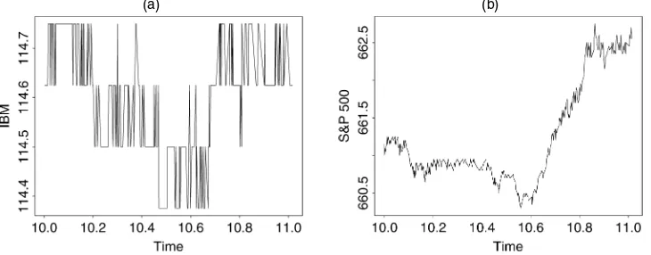
(a) (b)
Figure 1. Intraday Tick Graphs of, Respectively, IBM (a) and the S&P 500 (b) From 10AMUntil 11AMon February 12, 1996.
Kiesel (2001). These processes do not fit into the framework of this article. They violate our basic assumption of sample path continuity.
Ané and Geman (2000) fit a model of Gaussian returns to time-changed log returns for certain well-traded stocks such as IBM and Cisco. Because of the bid–ask spread, the tick data for these stocks show a characteristic square sawtooth effect and cannot be interpreted as sample functions of a continuous semimartingale; see Figure 1. Ané and Geman (2000) handled this difficulty by estimating the time change from the num-ber of transactions and showed that this is a better measure than the market volume used by Clark (1973). See also the article by Ané and Geman (1996), where the high-frequency data of one futures contract, for a period of 6 months, of the S&P 500 index is investigated. Florens, Renault, and Touzi (1998) tested whether financial processes are embeddable in stationary reversible continuous-time Markov processes. Al-though for certain stock indexes the embeddability is not re-jected, it is rejected for the daily return data of the S&P 500 stock index using daily data.
More recently a number of articles have focused on quadratic variation. We mention the articles by Andersen, Bollerslev, Diebold, and Labys (2000, 2001) on the realized volatility of foreign exchange rates. There is an important difference be-tween their approach and ours. We do not require independence between the time change and the price process. The assump-tion of independence implies that daily returns standardized by the daily realized volatility are iid standard normal variables. As pointed out by Andersen et al. (2003), daily standardized returns need not be iid standard normal if there is dependence between B andQ. If we standardize the daily returns of the S&P 500 index by the realized daily volatilities, we have to re-ject iid standard normality. This apparently is not the case for the foreign exchange data studied by Andersen et al. (2000) and the data studied by Ané and Geman (2000). Similar re-sults were reported by Peters and de Vilder (2002) for the main Dutch stock exchange index, using 15-second-interval data.
The rest of this article is organized as follows. Section 2 treats financial time. It consists of three parts. Section 2.1 discusses quadratic variation. Section 2.2 is concerned with increments of the log price process. Section 2.3 gives a detailed descrip-tion of the dataset and discusses the empirical time change. In Section 3 we perform a series of tests on the log price process
to test the hypothesis that the time-changed log prices of the S&P 500, corrected for drift, describe a sample function of Brownian motion. Section 4 analyzes the dependence between the price process and the time change. Section 5 contains some concluding remarks.
2. FINANCIAL TIME
This section treats financial time. In the first section, we shall describe the relationship between quadratic variation and finan-cial time. We discuss the difference between estimating the drift of a diffusion and its quadratic variation. In Section 2.2 we ana-lyze some of the statistical problems encountered in estimating financial time and the effects of using an estimate of financial time in normalizing the data. Section 2.3 is devoted to a de-scription of the dataset that we use in the analysis and to the construction of financial time for this dataset.
2.1 Quadratic Variation
The cornerstone result we use in this article is the time change for martingales theorem (Dambis 1965; Dubins and Schwartz 1965), which states the following. If Xis a continu-ous local martingale started at the origin, thenX=B◦Q, where Qis the quadratic variation of X andB is a standard Brown-ian motion. See Karatzas and Shreve (1991, thm. 4.6, p. 174). The converse implication holds if the random variablesQ(t)are stopping times forB. See Monroe (1978). So under the assump-tion that the quadratic variaassump-tion does not encode future events, the tests of this article validate the proposition that the S&P 500 futures index is a semimartingale and that model (1) holds.
To see how subtle this result is, we focus on two extreme cases. The first case is the classical problem of estimating a continuously differentiable drift functionf given the sample functionψ=f +ϕ over the interval[0,c], withϕ a standard Brownian sample function. For simplicity, assume the drift is linear,f(t)=at. Then the minimum variance unbiased estimate of the drift isaˆ=ϕ(c)/c. This estimator has a normal N(a,1/c)
distribution. Note, in particular, that the estimate is based on one observation only.
Now suppose we are given the functionx=ϕ◦q, whereqis an unknown continuous, strictly increasing function starting at the origin. Here the situation is completely different. Almost
every sample pathϕ of Brownian motion has the property that, given the distorted pathx=ϕ◦q, it is possible to reconstruct
ϕandqfor any time changeq.
So it is possible to recover the exact form ofqin contrast to the drift functionf. Indeed, this observation relates to Merton (1980), who showed that errors in the estimators of variances decrease with increasing sampling frequency, whereas this does not hold for the mean.
The quadratic variation Q= X,X of a continuous mar-tingaleX on the time interval [0,c]may be approximated by step processesQn starting at 0 at times0=0 and with jumps
(X(si)−X(si−1))2 at the times 0=s0<s1<· · ·<sn=c.
Fisk’s theorem (see, e.g., Kallenberg 1997) gives simple con-ditions for convergence of the step processes Qn to Q. This
result is also valid for a semimartingaleY =A+X, with Aa continuous process of bounded variation andY,Y = X,X. In Barndorff-Nielsen and Shephard (2002), the distribution of Qn is derived for stochastic volatility models. In that
arti-cle it is also shown that the error betweenQnandQdecreases
with the square root of the number of observationsn.
2.2 Increments of the ProcessX
We are interested in two types of increments: standardized increments in physical time and increments in financial time. Most interest in the financial literature has been given to the first type of incrementsUi, which are defined as
Ui=
X(si)−X(si−1)
Q(si)−Q(si−1)
, (3) wheres0<· · ·<snare equidistant time points in physical time,
for example, market closing times. The increments in (3) are iid standard normal ifBandQare independent. IfBandQare dependent, then this need not hold. Indeed, ifXis a continuous martingale and the variablesUiare not iid standard normal, then
BandQare dependent. In that case, the distribution ofUiis not
known.
On the other hand, dependence betweenBandQdoes not in-fluence the law of the scaled increments ofXin financial time. The latter increments are constructed as follows. Define finan-cial timeτ as the value of the time changeQat physical timet. Letτ0<· · ·< τm be equidistant time points in financial time.
are iid N(0,1)random variables regardless of the dependence structure ofBandQ. Here the inverse processQ−1(τ )is defined as
Q−1(τ )=inf
t>0{Q(t) > τ}, andτ=τi−τi−1,i=1, . . . ,m.
If we replace the quadratic variationQby an approximating sum of squares, then the increments in (4) will be independent and symmetric, but the kurtosis may be smaller than that of the standard normal distribution, as can be seen from the following theoretical result.
in (4), whereτ is replaced by the approximating sumQi=
ni Q−1(τi)] are independent normal variables with zero mean.
Together with the linearity of Q and the equidistance of t(0i), . . . ,tn(ii), this implies that Bi has the same distribution as
It is straightforward to compute the second and fourth mo-ment ofBivia
the random variableBiconverges to a standard normal random
variable.
In practice, we are confronted with a finite number of ob-servations. For certain time intervals, the volatility is high and financial time runs so fast that there are only a few observa-tion points available in the corresponding interval in physical time; that is, ni is small. Proposition 1 provides some
intu-ition that in these cases the tails are thin compared to the tails of the normal distribution. We avoid this problem by choos-ing sufficiently large financial time intervals. Observe that the assumption of piecewise linear quadratic variation in Proposi-tion 1 implies piecewise constant volatility.
2.3 The Data and Some Notation
Our dataset is the U.S. Standard & Poor’s 500 stock index fu-tures (S), traded on the Chicago Mercantile Exchange (CME), for the period January 1, 1988, to September 1, 2001. We could
have included October 1987 and September 2001 in our analy-sis. However, the extremely high volatility in these periods would decrease the number of observations in the fixed finan-cial time intervals dramatically as pointed out in the previous section. The extra data might also disrupt the homogeneity of our dataset, while the advantage of a longer dataset is only mar-ginal. In total, we have 3,452 trading daysd(=1, . . . ,3,452), where a day starts at 9:30 and ends at 16:00 CET. We always use the futures contract with the shortest time horizon, it being the most actively traded contract. There are four expiration months: March, June, September, and December. So we start with the futures contract that expired on the third Friday of March 1988. We next use the futures contract that expired on the third Friday of June 1988, and so on. The last contract we use is the one that expired on the third Friday of September 2001. Hence, the con-tracts we use always have a time horizon of at most 3 months.
We use futures data rather than the S&P 500 cash index to avoid nonsynchronous trading effects which cause positive au-tocorrelation between successive observations; see Dacorogna, Gençay, Müller, Olsen, and Pictet (2001). As in the cash in-dex, there are bid–ask effects in the futures prices that induce negative autocorrelation between successive observations; see Figure 1. One may deal with this by taking larger time inter-vals. The shortest (integer) time intervals where these effects are no longer visible have a length of 2 minutes. We restrict our attention to these 2-minute time intervals. At this point, we also want to refer to the work of Aït-Sahalia, Mykland, and Zhang (2005) and Bandi and Russell (2003). These article give a the-oretical treatment on how to deal with microstructure effects in high-frequency data. Because we are dealing with a very liquid asset, the error term due to microstructures is relatively small.
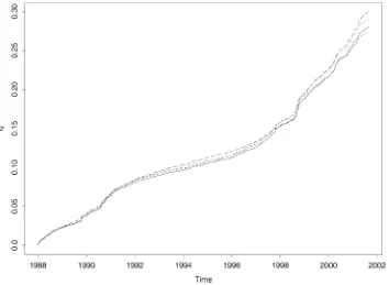
Figure 2 shows graphs of the estimates of the quadratic vari-ation for different time intervals and using all ticks. As ex-plained previously, the graph of the latter lies above the other
three graphs. The end values for the 2-, 4-, and 15-minute in-tervals vary only marginally. One can indeed show that the re-sults presented in this article do not depend on the choice of the 2-minute time intervals. However, increasing the length of the time intervals causes a rapid increase in the variance of the statistical error of the estimator ofQ; see Barndorff-Nielsen and Shephard (2002). This is hardly a desirable property and, hence, our choice of the 2-minute time intervals. In all four empirical functionsqˆ in Figure 2, different phases may be distinguished. The flatter parts correspond to periods where the financial clock runs slowly, whereas in the steeper parts the financial clock runs faster. Figure 2 also shows the graphs of the quadratic variation based on all ticks (top graph). The graph based on all ticks ends (at .3005) above the graphs based on the 2-, 4-, and 15-minute time intervals. These three graphs end at .2811, .2907, and .2751, respectively.
We have also computed the correlations between the daily increments of the four graphs. As expected, the correlations between the increments of the graphs based on 2, 4, and 15 minutes are high (between .90 and .95). On the other hand, the correlations of the increments of the graph based on all ticks and the increments of the graphs based on 2, 4, and 15 minutes are much lower (≈.6).
We assume that at each time point the S&P 500 futures has a value. The value is a real number. It changes continuously in time. It may be observed to a certain degree of accuracy by making a transaction in the futures contract. Transactions up-date the value. The small successive changes that we observe in the price of the futures contract may be the result of a com-plex underlying dynamical system. As in the physical Brownian motion of a pollen powhile suspended in water within certain bounds in time (increments over intervals of 2 minutes or more during a period of socioeconomic stability of 10 years), it may
Figure 2. Estimates of the Quadratic Variation Based on All Ticks at 2-, 4-, and 15-Minute Intervals. The end values are .3005, .2811, .2907, and .2751, respectively.
be possible to use a simple probabilistic model to describe the behavior. In our case, the complexity is hidden in the structure of the processQ(time change) and in the dependency between B and Q. The sole aim of this article is to test the hypothe-sis that the financial process associated with the process S is a time-changed Brownian motion. This seems to be ancicatial first step in the task of constructing a good model for financial processes.
Throughout this article, we shall use uppercase letters for random variables and lowercase letters for the corresponding realizations. The sample function of the process X is a con-struct. Each day yields jd +1=196 2-minute observations
s(d,0), . . . ,s(d,jd)and, thus,jdintervals. The observed
incre-mentz(d,j)of the processX over thejth interval of day d is defined as
z(d,j)=log
s(d,j) s(d,j−1)
−µ¯
jd
,
whereµ¯ is the average of the 3,452 daily log increments; see later. Now define
zd=z(d,1)+ · · · +z(d,jd),
(7)
σ2[d] =z2(d,1)+ · · · +z2(d,jd)
as the daily increase of the realization of the processXand the estimate of the realization of the daily increase of financial time, respectively. So the sample functionxof the processXand the estimate qˆ of the time changeQ associated with the sample functionxon time intervalst∈ [d−1+j/jd,d−1+(j+1)/jd)
are given by the (step functions) sums
x(t)=z1+ · · · +zd−1+z(d,1)+ · · · +z(d,j),
(8)
ˆ
q(t)=σ2[1] + · · · +σ[d−1]2+z2(d,1)+ · · · +z2(d,j).
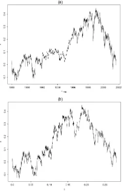
Notice that we focus on intraday prices. This is due to the absence of information on the quadratic variation during nights, weekends, and holidays. Hence, the processXis constructed in terms of a subset of increments of the “true” price process. This procedure does not affect the main point of this article because the sum of martingale increments is also a martingale. The sam-ple path of the resulting processXis shown in Figure 3.
The average return over the 3,452 days of our dataset equals
¯
µ≈7.23×10⁻⁵.
To evaluate the effect of the unknown drift termA(t)in (1) on our estimate qˆ of the quadratic variation, we assume that the functionAis smooth and that the slope ofAis on the order ofµ¯. The difference between the total quadratic variation ofx(t)and the total quadratic variation ofx(t)+ ¯µtequals
3,452×195(µ/¯ 195)2≈1.0×10⁻⁷.
Hence, the effect of a smooth drift function with slope on the or-der onµ¯ is on the order 10−7onqˆ(3,452)=.281. Such smooth drift functions have a negligible influence on the quadratic vari-ation.
The time pointsti where the processXis evaluated are
cho-sen according to a special rule. Becauseqˆ is a step function, we cannot choose the time pointsti so that τi=τi−τi−1, with τi = ˆq(ti), are exactly equal. Instead, we first fix τ
and then choose the time pointst1,t2, . . . successively so that
(a)
(b)
Figure 3. Log of the S&P 500 Corrected for Drift in Physical Time (a) and Log of the S&P 500 Corrected for Drift in Financial Time (b).
τi≥τ andτiis minimal. Thus,qˆ(ti)− ˆq(ti−1)≥τ and
ˆ
q(t′i)− ˆq(ti−1) < τ for any time pointt′i<ti. During periods
of high volatility,(τi−τ )/τ may be large. This error
be-comes larger asτ becomes smaller, causing additional noise in the observations ofBiin (4). One has to take this into account
when choosing the length of the financial time intervalτ. On the other hand, larger financial time intervalsτ decrease the number of observations, which, in turn, has a negative effect on the power of the tests used in this article. Taking these two considerations into account, we believe thatτ =.2ft, where ft=.001 units of financial time, is an acceptable, though ar-bitrary, choice. This gives us 1,372 financial time points con-structed, on average, with approximately 500 incrementsz. In physical time, this, on average, corresponds to one observation each 2.5 days. We emphasize that the results presented in this article apply equally well for different values ofτ. We have checked the results forτ =.1, .2, .5, and 1.0ft.
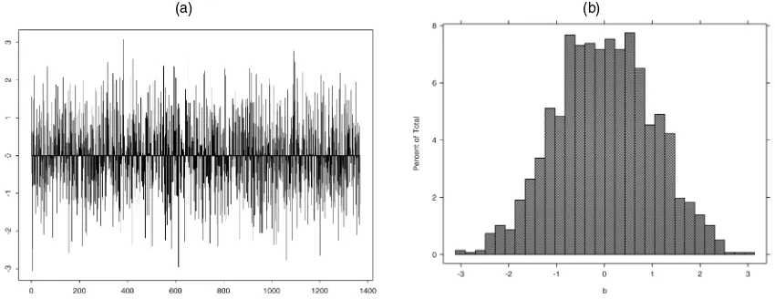
The scaled incrementsbiare given by
bi=
x(ti)−x(ti−1)
τi
and are depicted in Figure 4.
(a) (b)
Figure 4. Time Series of the Increments bi(a) and Its Histogram (b).
Figure 3(b) depicts the processXof the S&P 500 futures in-dex in financial time. Observe from this figure that patterns of the process in physical time [Fig. 3(a)] are conserved, possibly in stretched or compressed form, in financial time. Only the hor-izontal axis is deformed. The exact way in which the patterns are transformed is determined by the time-change function de-picted in Figure 2.
Table 1 displays some of the basic statistical properties of the incrementsbi. The table also lists the corresponding statistical
properties of the nonstandardized intraday returnsrd=zd+ ¯µ.
Observe that the skewness ofbiis close to 0. On the other hand,
the kurtosis of the series is less than 3. Using (5), we have com-puted the expected average kurtosis
k∗=m−1
m
i=1 3ni
ni+2 ≈
2.95,
whereni denotes the number of observations needed to
con-struct bi. Hence, under the assumptions of Proposition 1, the
kurtosis, as compared to the kurtosis of the normal distribution, is scaled downward by approximately .05.
3. TESTING THE HYPOTHESIS
This section tests the validity of the continuous semimartin-gale hypothesis for the S&P 500 against the alternative of con-tinuous processes that are not semimartingales. We do this by checking whether the processXis a Brownian motion in finan-cial time. For a continuous functionϕ:[0,a] →R, it is not hard
to test whether it is a Brownian sample path. Choose a large in-tegerm. Now observe that for a standard Brownian motionB the scaled increments(ϕ(a(i)/m)−ϕ(a(i−1)/m))/√a/m,i= 1, . . . ,m,are independent standard normal random variables. So we shall test whether the sequencebi may be regarded as
a sample from a sequence of iid standard normal random vari-ables.
Table 1. Statistical Properties of the Returns
Series Mean Standard deviation sˆ kˆ Size
rd 7.23×10⁻⁵ 9.28×10⁻³ −.487 13.6 3,452
bi 1.39×10⁻³ 1.01 −.0130 2.71 1,367
NOTE: Statistical properties of intraday returnsrdand the standardized returns in financial timebi.
3.1 The Tests
There is a wide variety of tests that may be used to check for iid standard normality. We have chosen five fundamentally different basic tests. Two tests for normalitity, one for the tails, and two for independence. We also present some graphical evi-dence.
The Kolmogorov–Smirnov Test. The first test we use is the Kolmogorov–Smirnov test. See Shorack and Wellner (1986) for a detailed discussion. We test for normality with fixed mean (=0) and fixed variance (=1). The outcomes are presented in Table 2. We also apply the test to the intraday returnsrd. As can
be observed from Table 2, standard normality is not rejected for the seriesbi. It is rejected for the unscaled return seriesrd.
Note that the intraday returns are demeaned by using the sample mean rather than the true mean. Large deviations of the sample mean from the true mean may result in a substantial degree of undersizing of the Kolmogorov–Smirnov test. To de-termine the magnitude of deviation of our sample mean with the true mean, we observe that the latter has a natural lower bound of 0 and a realistic upper bound of the risk-free rate plus a risk premium for equities. Because we are dealing with intraday re-turns, we roughly approximate the upper bound to be .05 on a yearly basis for our dataset. From Table 1, it follows that the annualized sample mean is approximately .02 with a standard error of .04. Hence, we do not expect to find large deviations between the true mean and the sample mean: We do not expect significant undersizing of the Kolmogorov–Smirnov test.
The Jarque–Bera Test. The Jarque–Bera (Bera and Jarque 1980) test exploits the skewness, ˆs, and the kurtosis, ˆk, from the empirical sequence and checks whether they can be dis-tinguished from the skewness and the kurtosis of a normal distribution with unknown mean and variance. The results of
Table 2. Testing for Normality
Series ks P( KS>ks) jb P( JB>jb)
rd .0624 .000 1.63×10⁴ .000
bi .0203 .629 4.87 .087
NOTE: The test statistics of the Kolmogorov–Smirnov (KS), Jarque–Bera (JB), and adjusted Jarque–Bera (JB∗) tests applied to the intraday log returnsrdand the seriesbi. For the seriesrd, we used a KS test with unknown mean and variance for the seriesbiwith fixed mean (=0) and variance (=1). We have also included thepvalues for the different statistics.
Table 3. Observations in the Tails together with the mean (µc), the standard deviation (σc), and the corresponding probabilities
P(Bc>nc), whereBcis Binomial(1,367,pc) distributed.
this test may also be found in Table 2. If we take into ac-count the expected value of the kurtosis k =k∗ <3, then the Jarque–Bera statistic n6(sˆ2+ 41(kˆ −3)2) is replaced by
(2n/3)(sˆ2+(ˆk−k∗)2)/4. Asymptotically, this Jarque–Bera sta-tistic isχ2distributed with 2 degrees of freedom. The corrected statistic has apvalue of .194 as compared to .087. Of course, the latter analysis is of a heuristic nature. Formally, a more thor-ough treatment is required. For reasons of brevity, we omit this exercise here.
As a final remark, we want to mention that one could also test for normality with fixed variance as in Bontemps and Meddahi (2005). Because the variance ofbi is close to 1, it is clear that
normality also cannot be rejected in that approach.
Hence, we cannot reject normality for the seriesbi. As
ex-pected, standard normality is rejected for the unscaled seriesrd.
The Binomial Test. Extreme values are important when dealing with financial data. We perform three simple binomial tests to check whether the seriesbi has heavy tails by
count-ing the number of observations exceedcount-ing the values of 2, 3, and 3.5 standard deviations, respectively. Letpc=P{|U|>c},
whereU is standard normal. For n independent observations of |U|, the number Nc of observations exceeding the level c
has a binomial-(n,pc) distribution with mean µc=npc and
varianceσc2=npc(1−pc). The observed number of
observa-tions exceedingcisnc. The results are presented in Table 3. As
can be seen from the table, the hypothesis that the tails behave like those of a standard normal distribution is not rejected at a level of 10% for the seriesbi. Although we did not distinguish
between the two tails of the distribution in Table 3, we have checked that similar conclusions can be derived when testing the tails separately.
The BDS Test. Next, we check whether the standardized re-turn series are iid. There are several ways to do this. We have chosen the BDS test, introduced in the financial literature by Brock, Dechert, Scheinkman, and LeBaron (1987). This test has often been (mis)used to investigate the presence of determin-istic (chaotic) structures in empirical time series. See Takens
(1993) for an enlightening discussion on this matter. The BDS statistic has power against a wide variety of departures from iid processes. The BDS, which was originally derived from the correlation integral, is based on the following property of an iid sequence. Let x1, . . . ,xN be a time series and let yj be a
andǫ >0. The BDS test uses the difference of estimates of these two probabilities, Pˆ(|Yj−Yj′|< ǫ)−(Pˆ(|Xk−Xk′|<
ǫ))m. The estimatesPˆ(|Yj−Yj′|< ǫ)andPˆ(|Xk−Xk′|< ǫ)are
obtained by counting the number of vectorsyjof observations
and the number of observationsxjthat lie within anǫdistance.
Under the null hypothesis, the difference between the probabil-ities is approximately normally distributed.
We calculate the BDS statistic for different embedding di-mensionsmand distancesǫforbi; see Table 4. Thepvalues in
Table 4 for eachmandǫ were obtained by reshuffling the se-quencebi2,000 times, calculating for each reshuffled sequence
the BDS statistic and then counting the number of absolute val-ues that exceeded the absolute value of the corresponding sta-tistic. Observe from Table 4 that we cannot reject iid on any reasonable level.
(Partial) Autocorrelation Function. As a final check for iid, we investigate the (partial) autocorrelation function for the se-quencesbi. If the series are indeed iid then we expect the
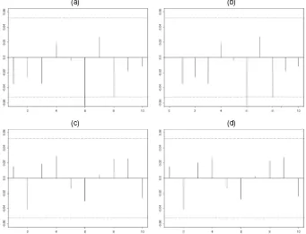
co-efficients of these functions to be close to zero. Figure 5 shows the autocorrelation functions forbifor lags of 1, . . . ,10 are
dis-played.
Observe from Figure 5 that for both functions only lag 6 lies outside the 95% confidence level. Moreover, the coefficients are, on average, negative. This is partly due to the fact that the process X, by construction, forms a Brownian bridge. Incre-ments of such processes are negatively correlated. The theoret-ical autocorrelation coefficient forbi is approximately−.001.
Therefore, we actually have to shift the confidence level down-ward by this number. Because this adjustment will not have a big impact on the results, we omit this exercise.
We next test whether the coefficients differ significantly from 0 by means of theQstatistic. TheQstatistic is defined
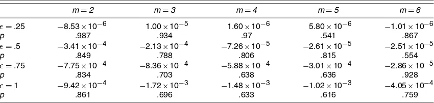
Table 4. The BDS Test
NOTE: The BDS statistics and the correspondingpvalues for the seriesbi. For embedding dimensionm=2, . . . ,6, each column contains the BDS statistic (bds) and thepvalue (p) for different values ofǫ. Thepvalues are obtained by reshufflingbi2,000 times, computing the BDS statistic for these new series, and then counting the number of absolute values exceeding the absolute value of bds ofbi.
(a) (b)
(c) (d)
Figure 5. Autocorrelation Function of the Increments bi for Lags 1–10 (a) and Partial Autocorrelation Function (b); Autocorrelation Function of
the Squared Increments bi2(c) and Partial Autocorrelation Function (d).
as
Q=T(T+2)
l
i=1 Ri
T−i,
whereRi is the estimator for the ith autocorrelation, l is the
number of lags, andTis the length of the time series. Under the null hypotheses, theQstatistic is asymptoticallyχ2distributed with 1 degree of freedom. We present the results in Table 5. Note that we cannot reject that thebiare realizations of an iid
sequence at the 10% level.
We performed the same analysis for the squared sequenceb2i. The bottom graphs in Figure 5 display the (partial) autocor-relation function for lags 1, . . . ,10. The corresponding Q sta-tistics are presented in Table 6. Note that we cannot reject independence for the squared sequence at the 10% level.
In addition to the tests described previously, we performed a number of qualitative graphical tests. Figure 6 displays the Gaussian kernel density estimate ofbiand the standard normal
density function. Observe that the two graphs have a large de-gree of resemblance.
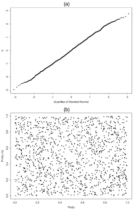
Figure 7 presents the quantile–quantile plot. As can be seen from this plot, most observations lie on the diagonal, which is an indication of the presence of normality. The points that devi-ate from the diagonal are accounted for by the slightly thinner
tails of the empirical distribution ofbias expressed by the
em-pirical kurtosisk∗(see Table 1) and the binomial test.
Figure 7 also depicts the scatterplot of((bi), (bi+1))for i=1, . . . ,1,366. Here denotes the standard normal distri-bution function. Observe that the transformed increments are uniformly distributed over the unit square. This finding is con-sistent with iid standard normality of the variables.
In summary, the statistical tests we have performed in this section on the realization of the processXin financial time show that the null hypothesis of a standard Brownian motion cannot be rejected. An alternative way to state the hypothesis is that in physical time the processX ofS is a time-changed Brownian motion. Under the assumption thatQdoes not contain informa-tion on future price changes, we cannot reject the hypothesis that the continuous semimartingale model in (1) for the S&P 500 holds.
4. DEPENDENCE BETWEEN FINANCIAL TIME AND THE PRICE PROCESS
In this section we investigate the dependence structure be-tweenQandB. Because in the previous section we have shown that we cannot reject the hypothesis that in financial time the
Table 5. Q Statistics of bi
Lags
1 2 3 4 5 6 7 8 9 10
q 1.69 2.51 3.98 4.62 4.64 10.21 11.38 14.8 15.0 15.2
p .197 .286 .260 .329 .461 .120 .123 .063 .091 .125
NOTE: Qstatistics (q) for lags 1–10 for the seriesbi. Thepvalues are denoted byp.
Table 6. Q Statistics of b2i
Lags
1 2 3 4 5 6 7 8 9 10
q .331 2.67 3.15 4.30 4.56 5.82 5.85 6.73 7.63 8.56
p .505 .264 .369 .366 .472 .444 .558 .566 .571 .574
NOTE: Qstatistics (q) for lags 1–10 for the seriesb2
i. Thepvalues are denoted byp.
processXis a Brownian motion, it is natural to define volatility over the interval[s,t]by
σ[s,t] =
Q(t)−Q(s)
t−s . (9)
Therefore, in our setting the squared volatility measures the speed of financial time with respect to physical time. Volatil-ity is high when the financial clock runs fast and low when the financial clock runs slowly.
Many studies present evidence that there is an asymmetric relationship between volatility and the price process; see, for example, Engle and Ng (1993). An appealing theoretical foun-dation for this relationship has been provided by Black (1976) and Christie (1982), who referred to it as thefinancial leverage effect. They reasoned that a decline in the stock price increases the company’s financial leverage, which makes the stock riskier and leads to a higher volatility level. A different but possibly complementary explanation for this asymmetric relationship is the so-called volatility feedback effect proposed by Pindyck (1984) and French, Schwert, and Stambaugh (1987). These au-thors argued that anticipated changes in volatility affect the re-quired return on the investment, which implies an immediate adjustment of the stock price. Although the previously men-tioned studies were concerned primarily with the behavior of individual stocks, it seems reasonable to assume that similar ar-guments apply to weighted sums of individual stocks. For an extensive study and discussion of both effects, see Wu (2001).
As indicated in Section 2.2, a clear indication thatBandQ are dependent would be that the standardized daily observations
u[d] =z[d]/σ[d] (10) are not realizations of an iid N(0,1) sequence. Here σ[d] stands for the daily volatility; see (7) and (9). Indeed, the mean (=.056), the variance (=.940), and the skewness (=.147) of
Figure 6. Gaussian Kernel Density Estimate of the Increments bi.
The dashed line corresponds to the standard normal density.
the series u[d] differ significantly from 0, and standard nor-mality has to be rejected. Hence, we conclude that B andQ are dependent. These findings seem to be in contradiction with those reported by Andersen et al. (2000) and Ané and Geman (2000), who presented evidence that foreign exchange rates and two individual stock returns, respectively, normalized by the daily volatilities, are Gaussian. Concerning the foreign ex-change rates, there is a priori no reason to assume that standard-ized returns and volatility are dependent. This is not obvious for asset prices.
Therefore, if the processXis a continuous martingale, then in physical time the standardized returns of an asset need not be iid standard normal, whereas scaled returns in financial time will be iid normal.
Let us now investigate the dependence structure that causes the rejection of iid standard normality for daily standardized returns. We focus on the relationship between the incrementsbi
(a)
(b)
Figure 7. Quantile–Quantile Plot of the Series bi(a) and Scatterplot
of (Φ(bi),Φ(bi+1)) (b). HereΦdenotes the standard normal
distribu-tion funcdistribu-tion.
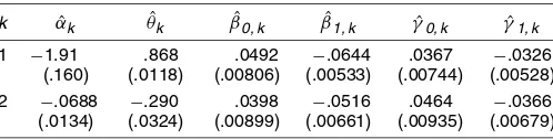
Table 7. Dependence Relationship
k αˆk θˆk βˆ0, k βˆ1, k γˆ0, k γˆ1, k
1 −1.91 .868 .0492 −.0644 .0367 −.0326
(.160) (.0118) (.00806) (.00533) (.00744) (.00528)
2 −.0688 −.290 .0398 −.0516 .0464 −.0366
(.0134) (.0324) (.00899) (.00661) (.00935) (.00679)
NOTE: The MLH estimates of the parameters in the regression relationship (11). The standard errors of the estimates are given in parentheses.
and the volatilityσi=σ[ti−1,ti]on the intervals[ti−1,ti]. The
time pointstiwere defined in Section 2.3, whereτi= ˆq(ti),i=
0, . . . ,1,366, are fixed financial time points.
We investigate the relationship by considering the regres-sions of logσi and log(σi/σi−1)on the first lag [logσi−1 and
Table 7 presents the estimates of the coefficients. Observe that both regressions have an identical form and that allγ’s have negative estimates. These findings show that, on average, the speed of financial time is higher for negative incrementsbi.
Financial time speeds up when increments are negative. This is evidence that the relationship between the price process and financial time is asymmetric.
5. CONCLUSIONS
The aim of this article was to test the semimartingale hypoth-esis for the S&P 500 stock index during the period 1988–2001 under the assumption of sample path continuity. In this hypoth-esis, the processX associated with the stock index is a con-tinuous martingale. The time change for martingales theorem states that any continuous local martingale is a time-changed Brownian motion. The time change is given by the quadratic variation of the process X. The estimate of the sample func-tion of the quadratic variafunc-tionQassociated with the 2 million data points for the S&P 500 futures is presented in Figure 2. It suggests that volatility over the 12-year period under consider-ation is not constant, but also that a constant volatility will give a reasonable first-order approximation to the processX deter-mined by the log returns, corrected for linear drift. Using this time change, we could not reject the hypothesis that in finan-cial time the processXis a standard Brownian motion against the compound alternative of a process with continuous sample paths. More precisely, we could not reject the hypothesis that the scaled increments, over fixed financial time intervals, of the processXare iid standard normal variables. On the other hand, the hypothesis that daily standardized increments are iid stan-dard normal is rejected. So there is significant dependence be-tween the time change and the Brownian motion. This is also
indicated by the estimates of the coefficients in the regression presented in (11).
ACKNOWLEDGMENTS
An earlier version of this article appeared in the DELTA (Paris, France) Research series 2002-06 (2002). The authors are indebted to the editor Torben Andersen, an associate editor, two anonymous referees, Guus Balkema, Nick Bingham, and Nour Meddahi for detailed comments and suggestions. R. Peters gratefully acknowledges the financial support of AOT N.V.
[Received February 2004. Revised January 2006.]
REFERENCES
Aït-Sahalia, Y. (2002), “Telling From Discrete Data Whether the Underlying Continuous-Time Model Is a Diffusion,”Journal of Finance, 57, 2075–2112. Aït-Sahalia, Y., Mykland, P., and Zhang, L. (2005), “How Often to Sample a Continuous-Time Process in the Presence of Market Microstructure Noise,”
Review of Financial Studies, 18, 351–416.
Andersen, T., Benzoni, L., and Lund, J. (2002), “An Empirical Investiga-tion of Continuous-Time Equity Return Models,”Journal of Finance, 57, 1239–1284.
Andersen, T., Bollerslev, T., Diebold, F., and Labys, P. (2000), “Exchange Rate Returns Standardized by Realized Volatility Are (Nearly) Gaussian,” Multi-national Finance Journal, 4, 159–179.
(2001), “The Distribution of Realized Exchange Rate Volatility,” Jour-nal of the American Statistical Association, 96, 42–55.
(2003), “Modeling and Forecasting Realized Volatility,” Economet-rica, 71, 579–625.
Ané, T., and Geman, H. (1996), “Stochastic Subordination,”Risk, 9, 146–149. (2000), “Order Flow, Transaction Clock, and Normality of Asset Re-turns,”Journal of Finance, 55, 2259–2284.
Bachelier, L. (1900), “Théorie de la Spéculation,”Annales de l’Ecole Normale Supérieure, 3.
Bandi, F., and Russell, J. (2003), “Microstructure Noise, Realized Volatility, and Optimal Sampling,” working paper, University of Chicago.
Barndorff-Nielsen, O., and Shephard, N. (2000), “Modelling by Lévy Processes for Financial Econometrics,” inLévy Processes—Theory and Applications, eds. O. Barndorff-Nielsen, T. Mikosch, and S. Resnic, Boston: Birkhäuser, pp. 283–318.
(2002), “Econometric Analysis of Realized Volatility and Its Use in Estimating Stochastic Volatility Models,”Journal of the Royal Statistical So-ciety, Ser. B, 64, 253–280.
(2003), “Integrated OU Processes and Non-Gaussian OU-Based Sto-chastic Volatility Models,”Scandinavian Journal of Statistics, 30, 277–295. Bera, A., and Jarque, C. (1980), “Efficient Tests for Normality,
Heteroscedas-ticity, and Serial Independence of Regression Residuals,”Economic Letters, 6, 255–259.
Bingham, N., and Kiesel, R. (2001), “Modelling Asset Returns With Hy-perbolic Distributions,” in Asset Return Distributions, eds. J. Knight and S. Satchell, Oxford, U.K.: Butterworth–Heineman, pp. 1–20.
Black, F. (1976), “Studies of Stock Price Volatility Changes,” inProceedings of Business and Economic Statistics Section, American Statistical Association, pp. 177–181.
Bontemps, C., and Meddahi, N. (2005), “Testing Normality: A GMM Ap-proach,”Journal of Econometrics, 124, 149–186.
Brock, W., Dechert, W., Scheinkman, J., and LeBaron, B. (1987), “A Test for Independence Based on the Correlation Dimension,”Econometric Review, 3, 197–235.
Carr, P., Geman, H., Madan, D., and Yor, M. (1999), “The Fine Structure of As-set Returns: An Empirical Investigation,”Journal of Business, 75, 305–332. Chernov, M., Gallant, A., Ghysels, E., and Tauchen, G. (2002), “Alternative
Models for Stock Price Dynamics,” Working Paper 2002s-58, CIRANO. Christie, A. (1982), “The Stochastic Behavior of Common Stock Variances—
Value, Leverage and Interest-Rate Effects,”Journal of Financial Economics, 10, 407–432.
Clark, P. (1973), “A Subordinate Stochastic Process Model With Finite Variance for Speculative Prices,”Econometrica, 41, 135–155.
Dacorogna, M., Gençay, R., Müller, U., Olsen, R., and Pictet, O. (2001),An Introduction to High-Frequency Finance, London: Academic Press. Dambis, K. (1965), “On the Decomposition of Continuous Submartingales,”
Theory of Probability and Its Applications, 10, 401–410.
Dubins, L., and Schwartz, G. (1965), “On Continuous Martingales,” Proceed-ings of the National Academy of Sciences of the United States of America, 53, 913–916.
Engle, R., and Ng, V. K. (1993), “Measuring and Testing the Impact of News on Volatility,”Journal of Finance, 48, 1749–1778.
Florens, J., Renault, E., and Touzi, N. (1998), “Testing for Embeddability by Stationary Reversible Continuous-Time Markov Processes,” Economet-ric Theory, 14, 744–769.
French, K., Schwert, G., and Stambaugh, R. (1987), “Expected Stock Returns and Volatility,”Journal of Financial Economics, 19, 3–29.
Kallenberg, O. (1997), Foundations of Modern Probability, New York: Springer-Verlag.
Karatzas, I., and Shreve, S. (1991),Brownian Motion and Stochastic Calculus, New York: Springer-Verlag.
Mandelbrot, B. (1963), “The Variation of Certain Speculative Prices,”Journal of Business, 36, 394–419.
Merton, R. (1980), “On Estimating Expected Returns on the Market,”Journal of Financial Economics, 8, 323–361.
Monroe, I. (1978), “Processes That Can Be Embedded in Brownian Motion,”
The Annals of Probability, 6, 42–56.
Peters, R., and de Vilder, R. (2002), “The Realized Volatility of the Main Dutch (AEX) Stock Index,” KdV Preprint Series, Amsterdam.
Pindyck, R. (1984), “Risk, Inflation, and the Stock Market,”American Eco-nomic Review, 74, 334–351.
Rosenberg, B. (1972), “The Behavior of Random Variables With Nonstationary Variance and the Distribution of Security Prices,” unpublished manuscript, University of California at Berkeley.
Shorack, G., and Wellner, J. (1986),Empirical Processes With Applications to Statistics, Chichester, U.K.: Wiley.
Takens, F. (1993), “Detecting Nonlinearities in Stationary Time Series,” Inter-national Journal of Bifurcation and Chaos in Applied Sciences and Engi-neering, 3, 241–256.
Wu, G. (2001), “The Determinants of Asymmetric Volatility,”The Review of Financial Studies, 14, 837–859.