Full Terms & Conditions of access and use can be found at
http://www.tandfonline.com/action/journalInformation?journalCode=ubes20
Download by: [Universitas Maritim Raja Ali Haji] Date: 12 January 2016, At: 23:32
Journal of Business & Economic Statistics
ISSN: 0735-0015 (Print) 1537-2707 (Online) Journal homepage: http://www.tandfonline.com/loi/ubes20
Standard Errors as Weights in Multilateral Price
Indexes
Robert J Hill & Marcel P Timmer
To cite this article: Robert J Hill & Marcel P Timmer (2006) Standard Errors as Weights in Multilateral Price Indexes, Journal of Business & Economic Statistics, 24:3, 366-377, DOI: 10.1198/073500105000000270
To link to this article: http://dx.doi.org/10.1198/073500105000000270
View supplementary material
Published online: 01 Jan 2012.
Submit your article to this journal
Article views: 48
Standard Errors as Weights in
Multilateral Price Indexes
Robert J. H
ILLSchool of Economics, University of New South Wales, Sydney 2052, Australia (r.hill@unsw.edu.au)
Marcel P. T
IMMERFaculty of Economics, University of Groningen, 9700 Av Groningen, The Netherlands (m.p.timmer@rug.nl)
Various multilateral methods for computing price indexes use bilateral comparisons as their basic building blocks. Some give greater weight to those bilateral comparisons deemed more reliable. However, none of the existing reliability measures adjusts for gaps in the data. We show how the standard errors on bilateral price indexes derived using weighted least squares provide reliability measures that solve this problem. We then apply our methodology to a dataset on agricultural production in 103 countries. Our results demonstrate the appeal of weighted methods and the importance of using weights based on a comprehensive measure of reliability.
KEY WORDS: International Comparisons Program; Multilateral price index; Reliability measure; Spanning tree; Stochastic approach; Weighted-Eltetö–Köves–Szulc.
1. INTRODUCTION
Comparing price levels and living standards across coun-tries is an issue of interest to national governments, firms, households, and international organizations such as the Interna-tional Monetary Fund, World Bank, and European Union. Such comparisons can influence budget contributions to international organizations and the allocation of aid flows. Relative price lev-els, or purchasing power parities, are best known for their use in obtaining international comparisons of GDP per capita, such as in the Penn World Table (see Summers and Heston 1991). They enable comparisons of productivity levels across coun-tries, which allow policy makers and firms to benchmark do-mestic performance. These comparisons are also relevant to the fields of development and international economics and to the literature on economic convergence.
Purchasing power parity (PPP) indexes are built from prices and quantities for a set of products in different countries and can be either bilateral or multilateral. Bilateral indexes, such as the Fisher index, have the disadvantage of being intransi-tive; that is, they do not generate internally consistent results for comparisons involving three or more countries. Transitiv-ity is achieved only when using multilateral methods. A num-ber of multilateral methods have been proposed in the index number literature. A distinction can be drawn between meth-ods that use bilateral comparisons as their basic building blocks and those that do not (see Hill 1997). Methods in the former category include the Eltetö–Köves–Szulc (EKS) and minimum spanning tree (MST) methods; methods in the latter category include the Geary–Khamis method. The PPP currency conver-sion rates used by the Penn World Table are computed using the Geary–Khamis method.
One attraction of building up a multilateral comparison from bilateral comparisons is that this approach opens up the pos-sibility of discriminating between bilateral comparisons on the basis of their reliability, giving greater weight to those deemed more reliable. For example, a comparison between France and Germany may be considered more reliable than one between France and India, because there is a greater overlap in the prod-ucts bought in France and Germany and because the prices and
consumption levels of the products consumed by both countries are more similar, thus making the comparison less sensitive to the choice of the index number formula. This observation pro-vides the underlying rationale for both the weighted-EKS (see Rao 1999) and MST (see Hill 1999) methods; however, both methods require that the reliability of bilateral comparisons be quantified.
In a survey of the literature on reliability measures, Rao and Timmer (2003) concluded that the main problem of existing measures, such as Hill’s (1999) Paasche–Laspeyres spread and Diewert’s (2002) class of relative price dissimilarity measures, is that they fail to make adjustments for gaps in the data. Rao and Timmer drew a distinction between statistical and index theoretic measures of reliability. The former take a sampling perspective; bilateral comparisons based on a small number of matched product headings or a low coverage of total expen-diture or production (averaged across the two countries) are deemed less reliable. In addition to the standard statistical ar-guments regarding small samples and a low coverage not be-ing representative, little overlap in the product headbe-ings priced by the two countries implies that they are very different and, by implication, inherently difficult to compare. Index theoretic measures, in contrast, focus on the sensitivity of a bilateral com-parison to the choice of price index formula. Most of the re-liability measures proposed in the literature, including Hill’s (1999) Paasche–Laspeyres spread and Diewert’s (2002) class of relative price dissimilarity measures, are of this type. Although these measures perform well when there are few gaps in the data, they can generate highly misleading results when there are many gaps. This is because they fail to penalize bilateral comparisons made over a small number of matched headings. It is precisely for such datasets that weighted methods are po-tentially the most useful, but only if they are able to combine the statistical and index theoretic criteria.
© 2006 American Statistical Association Journal of Business & Economic Statistics July 2006, Vol. 24, No. 3 DOI 10.1198/073500105000000270
366
The objective of this article is to develop such a measure. We depart from the existing literature, which is typically couched in an axiomatic setting, by approaching the problem from a sto-chastic perspective. We show how standard errors on the log-arithms of Törnqvist price indexes, derived from a stochastic model, provide a natural index theoretic measure of reliability that automatically penalizes bilateral comparisons with small overlaps of headings. We argue, therefore, that using standard errors as reliability measures will improve the quality of the re-sults generated by weighted-EKS and MST.
We conclude the article with an empirical comparison of our reliability measure and its resulting weighted-EKS and MST price indexes with those obtained using other measures. The dataset from the United Nations (UN) Food and Agriculture Organization (FAO) comprises of agricultural producer prices and quantities for 181 agricultural crops covering 103 coun-tries. The interesting feature of the dataset from our perspective is that it covers a large and diverse set of countries and contains many gaps. The presence of gaps in such a dataset is inevitable; for example, it is not surprising that tropical foods and spices are not grown in Norway. If we want to find the most reliable bi-lateral comparisons in this dataset, it is crucial that we take into account the amount of overlap of crops in each bilateral com-parison. We show that the failure to make such adjustments can lead to a highly undesirable allocation of weights, thus com-promising weighted binary-based multilateral methods, such as weighted-EKS and MST, in precisely those situations where they are most needed.
2. BILATERAL AND MULTILATERAL PRICE INDEXES
2.1 Bilateral Price Indexes
The set of countries is indexed byk=1, . . . ,K, and the set
of commodity headings is indexed byn=1, . . . ,Njk. Here we
allow for the possibility that the set of headings over which each bilateral comparison is made may not be identical. This is the
reason for thejksubscript onN. The price and quantity data of
headingnin countrykare denoted bypknandqkn.
LetPjkandQjkdenote bilateral price and quantity index
com-parisons between countriesjandk. Four important bilateral
in-dex number formulas are defined as follows (with the history of these formulas discussed in Diewert 2001):
Laspeyres: PLjk=
One weakness of these formulas is that they are not transitive; for example, in general,PFjk×PFkl=PFjl.
2.2 Multilateral Price Indexes
A multilateral price index, by construction, is transitive.
Mul-tilateral price indexes for countriesjandkare denoted herein
by Pj andPk. A bilateral comparison of prices made using a
multilateral formula can be expressed as
Pjk=
Pk
Pj
.
Transitivity is achieved by sacrificing the independence of
irrel-evant alternatives (see van Veelen 2002). That is, the ratioPk/Pj
in general will depend not only on the price and quantity vectors
of countriesjandk, but also on the price and quantity vectors
of some or all of the other countries in the comparison. A large number of multilateral formulas have been proposed in the in-dex number literature (see, e.g., Balk 1996; Hill 1997; Diewert 1999; Cuthbert 2000 for surveys of this literature).
3. BINARY–BASED MULTILATERAL METHODS
Binary-based multilateral methods are constructed by com-bining bilateral comparisons between pairs of countries. Here we consider four binary-based multilateral methods. The first method weights the bilateral comparisons in an arbitrary way, whereas the second gives equal weight to all bilateral compar-isons. The third and fourth methods give greater weight to those bilateral comparisons deemed more reliable. It is these latter methods that are the focus of attention here, because their per-formance depends critically on the way reliability is measured.
3.1 Star Methods
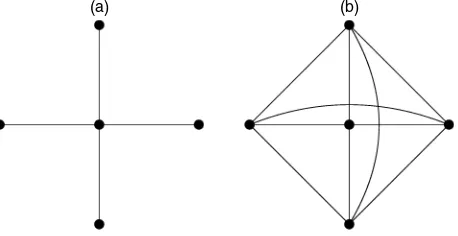
Graph theory provides a useful framework for analyzing the underlying structure of binary-based multilateral price indexes. A graph consists of a collection of vertices linked by edges. In the context of spatial comparisons, each vertex represents one of the countries in the comparison, and each edge represents a bilateral comparison between a pair of countries. Two particu-larly important graphs, depicted in Figure 1 for the case of five vertices, are the star and complete graphs.
Perhaps the simplest multilateral method is the star method, which uses the star graph. The star method places one
coun-try, denoted here byb, at the center of the star. The multilateral
price index for country k is then defined asPk=Pbk, where
Pbkis a bilateral price index, such as the Fisher or Törnqvist
in-dex. This means that a comparison between countriesjandkis
made by linking together bilateral comparisons between
coun-triesjandband countriesbandk.
(a) (b)
Figure 1. Examples of Graphs: (a) Star Graph; (b) Complete Graph.
But the fact that the bilateral formulas are not transitive im-plies that the multilateral price indexes depend on which coun-try is placed at the center of the star. For example, suppose that
countrybis replaced with countrydat the center of the star. In
general, then,
This is the main weakness of the star method. In most applica-tions, it is not clear which country should be placed at the cen-ter of the star. Such methods as those of Geary (1958), Khamis (1972), and Iklé (1972) solve this problem by putting an artifi-cial average country at the center of the star. As a result, neither of these approaches is binary-based.
3.2 The EKS Method
The EKS method, named after Eltetö and Köves (1964) and Szulc (1964) but first proposed by Gini (1931), also uses the star graph. It manages to treat all countries symmetrically by
generating K series of multilateral price indexes, each with a
different country at the center of the star. These K series of
results are then averaged. The EKS method usually uses the Fisher index to make the bilateral comparisons. The Törnqvist version of EKS is often referred to as the CCD method (Caves, Christensen, and Diewert 1982). One attractive feature of the CCD method is that it can also be represented as a star method with an artificial country at the center of the star. The EKS for-mula transitivizes the bilateral price indexes as
Pk=
EKS is the preferred multilateral method of Eurostat and the OECD.
The EKS method can also be described using a complete graph (see Fig. 1), because it uses bilateral comparisons
be-tween all possible pairs of countries. A total of K(K−1)/2
distinct bilateral comparisons are defined on a set ofKvertices.
Inevitably, some of these bilateral comparisons are likely to be more reliable than others. This observation provides the ratio-nale for the weighted-EKS method discussed next.
3.3 The Weighted-EKS Method
The weighted-EKS method, proposed by Rao (1999) and dis-cussed in greater detail by Rao (2001) and Rao and Timmer
(2003), allows each bilateral comparison to be given different weight in the multilateral comparison. The EKS price indexes
Pj andPk can be obtained as the solution to the minimization
problem
where the normalization P1=1 is imposed. The solutions,
lnPˆj and lnPˆk are the ordinary least squares estimators of
lnPjand lnPkin the model
lnPFjk=lnPk−lnPj+ǫjk, (6)
withE(ǫjk)=0 and var(ǫjk)=σ2.
Rao’s weighted-EKS method assumes instead that the errors are heteroscedastic, that is,
var(ǫjk)=σ2/wjk forj=k and var(ǫjj)=0. (7)
The weights,wjk, measure the reliability of the comparison
be-tween countriesjandk. We discuss specification of thewjklater
in the article. For now, we treat them as given. The complete
matrix of weights is denoted here byW. The matrixWmust
be symmetric. In addition, if a particular bilateral comparison is assigned a weight of 0, then in (7) this comparison should be interpreted as having an infinite variance. Hence it plays no part in the determination of the weighted-EKS price indexes,
W=
The weighted-EKS price indexes,Pk, are obtained as
The price index for country 1,P1, is normalized to 1. In the
case wherewjk=wfor alljandk, the weighted-EKS method
reduces to the standard EKS formula in (5).
3.4 The Minimum Spanning Tree Method
A multilateral comparison betweenKcountries can be made
by simply chaining togetherK−1 bilateral comparisons (i.e.,
edges), as long as the underlying graph is aspanning tree(see
Hill 1999). A spanning tree is a connected graph that does not contain any cycles. In other words, any two vertices in the graph are connected by one and only one path of edges. The rea-son why there must be no cycles in the graph is to ensure that the multilateral price indexes are transitive and hence internally
consistent. A total ofKK−2different spanning trees are defined
on a set ofKvertices. Three examples of spanning trees defined
on the set of nine vertices are shown in Figure 2. The star graph in Figure 1 is another example of a spanning tree.
The resulting set of multilateral price indexes depends on both the choice of formula for making the bilateral compar-isons and the choice of spanning tree. The bilateral comparcompar-isons should be made using a superlative formula, such as Fisher or Törnqvist. (See Diewert 1976 for a definition and discussion of the properties of superlative indexes.) Because superlative
for-mulas satisfy the country reversal test (i.e.,Pjk=1/Pkj), there
is no need for directional arrows on the edges in the spanning tree to identify the base country in each bilateral comparison.
The choice of spanning tree is more problematic. A criterion is needed for deciding which edges (i.e., bilateral comparisons) to include and which to exclude. As with the weighted-EKS method, this requires that a weight be placed on each bilateral comparison. Again, the specification of weights is deferred un-til later. In the context of the MST method as described by Hill (1999), however, it should be noted that the greater the reliabil-ity of a bilateral comparison, the smaller its reliabilreliabil-ity measure. The MST method can be easily reformulated so that reliabil-ity is an increasing function of the reliabilreliabil-ity measure, as is the case in the weighted-EKS method. Given this setup, it is the maximum-spanning tree, not the minimum-spanning tree that is required.
The maximum spanning tree can be derived using Kruskal’s algorithm. Kruskal’s algorithm proceeds by selecting sequen-tially the bilateral comparisons (edges) with the largest weights subject to the constraint that adding that edge to the graph does not create a cycle. The algorithm terminates once it is no longer possible to select any more edges without creating a cycle. It turns out that the resulting spanning tree has the maximum sum
of weights. This is a well-known theorem in the graph the-ory literature (see, e.g., Wilson 1985). In some sense, the MST method can be considered a special case of the weighted-EKS
method for which 2(K−1)of the elements of theWmatrix are
set equal to 1 and all other elements equal 0.
4. A SURVEY OF EXISTING MEASURES OF RELIABILITY FOR BILATERAL COMPARISONS
Both the weighted-EKS and MST methods require the con-struction of a matrix of weights. Ideally, we should use what-ever bilateral comparisons are most reliable. One important difference between the two methods is that MST price indexes depend only on the ordinal ranking of the reliability measures. Hence MST price indexes, unlike weighted-EKS price indexes, are unaffected by monotonic transformations of the reliabil-ity measure. For example, the logarithmic transformation of the PLS measure defined in (8) matters for the weighted-EKS method but is of no consequence for the MST method.
The literature on reliability measures for bilateral compar-isons has been developed for the most part in an axiomatic setting. When discussing the sensitivity of a bilateral compar-ison to the choice of index number formula, it is useful to first consider the limiting cases where all formulas give the same answer. The data are consistent with the conditions for
Hicks’ aggregation theorem (Hicks 1946) if pkn=λpjn for
n=1, . . . ,Njk, whereλdenotes a positive scalar. In this case all
price index formulas reduce toλ. The data are consistent with
the conditions for Leontief’s aggregation theorem (Leontief
1936) ifqkn=µqjnforn=1, . . . ,Njk, whereµagain is a
posi-tive scalar. In this case all quantity index formulas reduce toµ.
It follows, therefore, that all price index formulas should
re-duce to(Njk
n=1pknqkn)/(µ
Njk
n=1pjnqjn), because price indexes
can be obtained implicitly from quantity indexes.
One measure of sensitivity that has received attention in the index number literature is the Paasche–Laspeyres spread (PLS), usually defined as some function of the ratio of a Paasche price index to a Laspeyres price index. (The ratio of Paasche to Laspeyres is the same for price and quantity indexes.) For example, Hill (1999) defined it as
PLSjk=ln
max(PP
jk,PLjk) min(PPjk,PLjk)
. (8)
The PLS has the attractive property of equaling 0 if the data satisfy the conditions for either Hicks or Leontief aggregation. When either condition is satisfied, there is no index number
Figure 2. Examples of Spanning Trees.
problem, because all formulas should give the same answer. This suggests that we can have a high degree of confidence in the results of a bilateral comparison with a small PLS, because the underlying data are broadly consistent with either Hicks or Leontief aggregation. However, the link between the PLS and Hicks or Leontief aggregation is not exact, because the PLS can equal 0 even when the conditions for Hicks and Leontief aggre-gation are both violated.
For this reason, Diewert (2002) advocated separate measures of sensitivity for price and quantity indexes, which he referred to as “relative dissimilarity measures.” He considered the ax-iomatic properties of a number of alternative measures. His rel-ative dissimilarity measures for prices (quantities) all share the characteristic that they equal 0 if and only if the data satisfy the conditions for Hicks (Leontief ) aggregation. One of his pre-ferred measures is
where SPjk andSQjk denote the price and quantity dissimilarity
measures andPTjkandQTjkdenote Törnqvist price and quantity
indexes as defined in (4).
If desired,SPjkandSQjkcan be combined as
Sjk≡min(SPjk,S Q
jk). (11)
This measure, a variant of which was used by Hill (2004), equals 0 if and only if the data are consistent with either
Hicks or Leontief aggregation. For most datasets,SPjk<SQjk, and
hence Sjk will simplify to SPjk. This empirical regularity was
noted by Allen and Diewert (1981). It is worth noting that when
Njk=1 (i.e., the comparison is made over only one heading),
PLSjk=SPjk=S Q
jk=Sjk=0. Thus, for the measure to be
mean-ingful, we must restrict attention to cases whereNjk≥2.
All of the reliability measures discussed herein, however, share one fundamental weakness: They all assume that there are no gaps in the data. As soon as there are gaps, this means that some bilateral comparisons will be made over larger bas-kets of products than others. All other things being equal, we should prefer bilateral comparisons made over larger baskets. Furthermore, the sheer fact that two countries have very little overlap in the products produced (or consumed) indicates that these countries are very different and, by implication, hard to compare. Therefore, ideally a measure of reliability should pe-nalize bilateral comparisons where the overlap of products is small. At first glance, it seems that any such adjustment must be arbitrary; however, by approaching the problem from a sto-chastic perspective, in the next section we derive a reliability measure that naturally makes such an adjustment. In addition, although we approach the problem from a very different per-spective than Diewert (2002), who used an axiomatic approach, it emerges that our reliability measure is a generalization of one of his measures.
5. A STOCHASTIC APPROACH TO THE MEASUREMENT OF RELIABILITY
In this section we show how when the same problem of mea-suring the reliability of bilateral comparisons is approached from the stochastic perspective, we obtain standard errors on the logarithms of Törnqvist price indexes that can serve as measures of the reliability of bilateral comparisons. Further-more, we link these standard errors with the existing litera-ture by showing that they are, in fact, generalizations of one of Diewert’s relative price dissimilarity measures. The main differ-ence is that the standard errors contain an additional term that penalizes bilateral comparisons where the overlap of products is small. This finding provides an interesting new link between the axiomatic and stochastic approaches to index numbers.
Our approach here is somewhat analogous to that used in the weighted country product dummy (WCPD) method (see Rao 2001; Diewert 2004a). Our approach specifies a stochas-tic model in price relatives in a bilateral setting, as opposed to WCPD, which specifies a stochastic model in price levels in a multilateral setting.
Our stochastic model builds on the work of Clements and Izan (1981), Cuthbert and Cuthbert (1989), and Selvanathan and Rao (1994). These authors showed how the stochastic ap-proach can be used to derive standard errors on the logarithms of Paasche, Laspeyres, and Törnqvist indexes, as functions of the number of observed price headings (see also Diewert 1995). Although they do not draw attention to this issue (which is not surprising because these articles predate Diewert 2002), it turns out that the standard errors on the logarithms of the Törnqvist price indexes derived by Clements and Izan (1981) and Selvanathan and Rao (1994) differ from Diewert’s
dissim-ilarity measureSPjk only in that they make as adjustment by
di-vidingSjkP byNjk−1. Hence these standard errors do make a
simple adjustment for gaps in the data. However, the adjustment is not entirely satisfactory because it does not take into account the value share of each product. Our model differs slightly from theirs and in the process generates a more satisfactory method of adjustment that explicitly factors in value shares. The ap-proach of Cuthbert and Cuthbert (1989) is slightly different again, in that it focuses on comparisons below the basic heading level. (Cuthbert and Cuthbert’s contribution is discussed later in the article.)
It is useful to begin with a discussion of Clements and Izan’s stochastic model of the Törnqvist price index. They assumed that the price relatives can be modeled as
ln
The termαjk in (12) represents the systematic part of the
dif-ference in the purchasing power of the currencies of countries
jandk, whereas εjk,n denotes the random element. Clements
and Izan assumed that the errors are independently distrib-uted as
E(εjk,n)=0, var(εjk,n)=
σjk2
Njkwjk,n
, (13)
wherewjk,n>0 denotes a nonrandom weight attached to
head-ingi, such thatNjk
n=1wjk,n=1. It is assumed thatNjk≥2. Also,
here we have addedNjkto the denominator of the variance term so that the harmonic mean of the variances across all headings is independent of the number of headings. This adjustment is needed to make the results consistent with a different version of the model discussed later.
The important point about Clements and Izan’s specification
is thatwjk,ndiffers across headings. The model presumes that
the price relatives of headings with larger weights (value shares) are measured with greater accuracy and hence more closely ap-proximate the underlying price index.
Continuing for the moment with our slightly modified version of the Clements and Izan model, it follows from
(12) and (13) that the generalized least squares estimator ofαjk
is
Törnqvist price index. It follows from (13) that
var(αˆjk)=
An unbiased estimator ofσjk2is
ˆ
Returning to (13), suppose that now we modify the underly-ing assumptions as
E(εjk,n)=0, var(εjk,n)=(σjk)2, (17) so that the variances of the errors are independent of the weights. We believe this assumption is more realistic, because the weights are later set equal to the average value shares, that
is,wnjk=(sjn+skn)/2. There is no reason to presume that
head-ings with larger value shares are measured more accurately. In fact, if anything, the reverse is likely to be true, as is illustrated by the examples of the health and education headings, which have large shares and are very hard to measure. Hence the as-sumption regarding the variance of the errors in (17) is defi-nitely an improvement on (13).
Our second departure from the approach of Clements and Izan is that instead of generalized least squares (GLS) in a heteroscedastic model, we use weighted least squares in a
ho-moscedastic model to estimateαjk, with the weight on
observa-tionnequal towjk,n,
that is, we give greater weight to those headings that have larger value shares, because they are more important in an economic sense. GLS, in contrast, gives greater weight to headings that are measured with greater accuracy. If it is assumed (unrealisti-cally in our opinion) that headings with larger value shares are measured more accurately, as in the Clements and Izan model, then it might seem that the two approaches are mathematically equivalent. But this is not the case. Although both approaches
lead to the same estimator ofαjk, the estimator’s variance
dif-fers in the two models.
Solving (18), we obtain the following estimator ofαjk:
˜
An unbiased estimator ofσjk2in our model is
˜
This result is derived as
E
Setting the weights equal to the average value shares,wjk,n=
(sjn+skn)/2, in (16) and (21), we obtain that
That is, the estimated variance is a function of Diewert’s relative
price dissimilarity measure,SPjk. Replacingσjkwithσˆjk in (15),
we obtain that
tion (25) provides a new measure of the variance of the loga-rithm of a Törnqvist price index.
It is important to consider the impact of Njk on var(αˆjk)
and var(α˜jk). It is not clear in general how an increase inNjk
(forNjk≥2) will affectSPjk. However, an increase inNjk must
calculated only over the products (headings) supplied by both
countries j andk (i.e., Njk
n=1sjn=
Njk
n=1skn=1). Hence, as
Njk rises, each of thesjnandsknterms, on average, should fall
which in turn should reduce the numerator and increase the
de-nominator of (25), thus causing var(α˜jk) to fall. The
empiri-cal analysis later in the article bears out these claims. Although
var(αˆjk)clearly penalizes (relative toSPjk) bilateral comparisons
with smaller overlaps, the adjustment takes no account of the relative importance in terms of value shares of each product. It
is for this reason that we believe var(α˜jk)to be a superior
mea-sure of reliability.
Quantity versions of the stochastic models in (13) and (17) could also be developed. However, in this context it is more natural to treat the prices as being stochastic and the quantities as responding to prices.
6. CHOOSING THE WEIGHTS
6.1 Above Basic Heading Level
It is useful to draw a distinction between applications of price index methods above and below basic heading level. Above ba-sic heading level, value shares are available, whereas below basic heading level, they are not. This distinction is relevant mainly to consumer datasets, such as those used by the Inter-national Comparisons Program (ICP), the OECD, and Eurostat, which rely on household expenditure surveys to obtain value shares.
Focusing first on comparisons above basic heading level (the usual case), if the Fisher index is replaced by Törnqvist in (6), and assuming heteroscedastic errors as in (7), we obtain the following model:
ance of the logarithmic deviations of Törnqvist price indexes from CCD price indexes in a multilateral comparison, whereas the latter is the variance of the logarithms of the price relatives
in a bilateral comparison between countriesjandk.
It follows from (26) that
var(lnPTjk)=var(ǫjk)=
σ2
wjk
.
Finally, using (25), we obtain the following weights for the weighted-EKS and MST methods:
wjk=
With the weights defined in this way, the MST method uses the
maximum spanning tree. The value ofσ2in (27) has no effect
on the resulting multilateral price indexes, and hence can be set equal to 1.
6.2 Below Basic Heading Level
Below basic heading level (i.e., at a level of detail lower than that provided in household expenditure surveys), value shares are not available. This distinction between above and below ba-sic heading level often arises in datasets covering consumer ex-penditures. The ICP, OECD, and Eurostat all have to construct price indexes at both levels.
A distinction can be drawn between cases where some prod-ucts are identified as representative for a particular country— an approach pioneered by Eurostat and further developed in the latest round of the ICP (see International Comparison Program 2005)—and cases where no such distinction is made. Consider-ing first the latter scenario, it follows thatwjk,n=1/Njkfor alln. Therefore, the Törnqvist index in (4) reduces to the Jevons in-dex (see Diewert 2004b), defined as
Jevons: PJjk=
Similarly, Diewert’s price dissimilarity measure defined in (9) reduces to
Equation (27) now reduces to
wjk=
σ2(Njk−1)
SPjk ,
whereSjkis defined as in (29).
Suppose now that each country identifies some products as
representative. Now letn=1, . . . ,Njk index the products that
are representative in either countryjorkand are priced in both
jandk. Also letNjkRdenote the number of products that are
rep-resentative in countryjand priced ink, whereasNRkjdenotes the
number of products representative in countrykthat are priced
inj.
The weights on each product can now be defined aswjk,n=
(s∗j,n+s∗k,n)/2, wheres∗j,n=1/NjkRif productnis representative in countryjand s∗j,n=0 otherwise. Similarly,s∗k,n=1/NkjR if
productnis representative in countryk, ands∗k,n=0 otherwise.
This means that any data available on a product that is not rep-resentative for either country is ignored, even if both countries price this product. If such a scenario is deemed unsatisfactory, then an alternative approach is to simply give greater weight to
representative products. For example, letNjkU denote the
num-ber of unrepresentative products in countryjthat are priced by
both countries. We could sets∗j,n=θ/(θNjkR+NjkU)if productn
is representative ands∗j,n=1/(θNRjk+NjkU)ifn is
unrepresen-tative, whereθ≥1 is a parameter that determines the relative
weight given to representative and unrepresentative products.
The greater the value ofθ, the smaller the weight given to
un-representative items. At one extreme, whenθ=1,
representa-tive and unrepresentarepresenta-tive products priced by both countries are treated symmetrically. At the other extreme, in the limiting case
asθtends to infinity, we obtain the previous model.
Using this approach, quasi-Törnqvist indexes can be
com-puted with sjn and skn replaced by s∗jn and s∗kn in (4). Using
these quasi-value shares, it is likewise possible to computeSPjk
and var(αˆjk), and hence the methodology becomes analogous to
the above basic heading case.
In a typical multilateral comparison, this process is repeated for each heading (expenditure class) of which there may be around 200. Therefore, although the standard procedure should work in most cases, there almost certainly will be a few
prob-lematic headings where either NjkR and NjkU, NkjR and NkjU, or
both will equal 0 in one or more of the bilateral compar-isons. Clearly, when this happens it is not possible to com-putePTjk,SPjk, and var(αˆjk), because the weights wjk,n are not defined. For the purposes of the weighted-EKS and MST
meth-ods, in such cases var(αˆjk) should be set to infinity. This
ensures that this bilateral comparison is completely ignored by both methods. If, for a particular heading, this situation arises for so many bilateral comparisons that it is not even possible to construct a spanning tree from the remaining com-parisons, then Törnqvist must be replaced by either
quasi-geometric Laspeyres or Paasche where required in the SPjk
formulas.
The stochastic properties of the quasi-Törnqvist index have been considered previously by Cuthbert and Cuthbert (1989), although, confusingly, they referred to this index as a Fisher index. (This terminology can be traced back to Eurostat.) Cuthbert and Cuthbert derived an expression for the variance of the quasi-Törnqvist index that corresponds to (20), with the
quasi-weights defined as earlier withθ set to infinity (see also
Rao 2001). But Cuthbert and Cuthbert did not derive an
estima-tor forσjk2for their stochastic model, and hence as it stands, the
variances cannot actually be computed (up to a scalar of
pro-portionality) unless it is assumed thatσjkis the same across all
bilateral comparisons.
7. EMPIRICAL APPLICATION TO AN AGRICULTURAL DATASET
The dataset consists of agricultural producer prices and quan-tities for 181 agricultural products (mainly crops) for the year 1995. Because quantities (and hence value shares) are available for each product, as is usually the case in producer datasets, the distinction between above and below basic heading level is not relevant. The weighting formula in (27) can be used di-rectly. The dataset covers 103 countries. It was constructed by Rao, Ypma, and van Ark (2003) from a UN FAO agricultural and producer prices database. We have slightly modified Rao et al.’s original dataset, which contained 111 countries, by re-moving 8 countries. We removed Singapore and Chad due to a very limited number of agricultural products, and removed six Central Asian countries for which the price data were not origi-nal but appeared to be imputed from the Ukraine. (See Rao et al. 2003 for a full description of the dataset.)
The interesting feature of the dataset from our perspective is that it contains many gaps. This is inevitable in a dataset that covers most of the crops grown in the world. For example, it is not surprising that tropical foods and spices are not grown in Norway. If we want to find the most reliable bilateral compar-isons in this dataset, it is crucial that we take into account the amount of overlap of crops in each bilateral comparison.
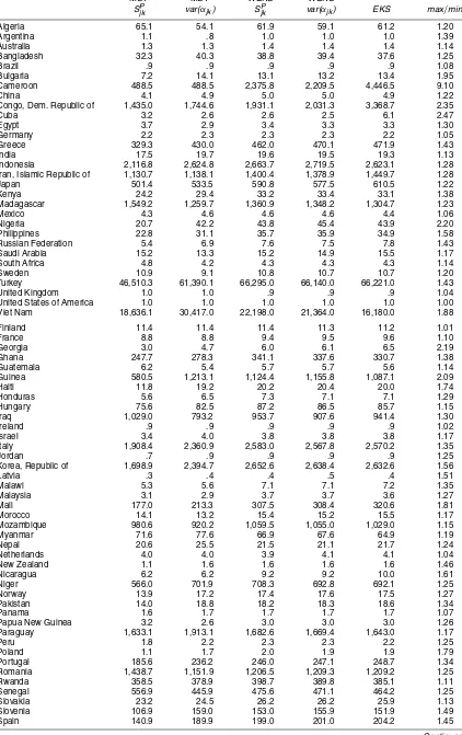
The bilateral comparisons selected by the MST method are particularly illuminating. A total of 102 bilateral comparisons are selected (by construction, one less than the number of coun-tries in the comparison). The top 25 bilateral links are listed
in Table 1 in descending order for Diewert’s measure, 1/SPjk,
and our measure, 1/var(α˜jk). The full list of 102 bilateral links
for each weighting scheme has been provided by Hill and Timmer (2004). It is immediately apparent that many of the
links for 1/SPjk are surprising. Some particularly eye-catching
links that were among the first 25 selected (i.e., the best bi-lateral links in the MST) are Norway–Niger (2), Norway– Malaysia (2), Norway–Indonesia (3), Malaysia–Canada (4), Mali–Georgia (4), and Ghana–Canada (2). The size of the
prod-uct overlap,Njk, is provided in brackets after each link. The fact
that these bilateral comparisons all have a low product over-lap indicates that they may not be reliable, and hence probably should not be used to construct a spanning tree or given high weights in the weighted-EKS method. Only two of these six
links are selected by our measure, 1/var(α˜jk), and in both cases
they are further down the list. The MST links obtained using our measure are intuitively more plausible. In addition, the average
value ofNjkis 27.6, as opposed to 14.2 for Diewert’s 1/SPjk
mea-sure. The difference is even more dramatic for the best 25 links.
The averageNjkfor this subset of links is 35.0 for our measure,
compared with 11.1 for 1/SjkP.
The problem with using weights based on 1/SjkPis that when
Njk is small, it will contain a lot of noise. This means that in
such cases, there is a chance that 1/SjkP could be large even
though, almost by definition, countriesj andk must be quite
different. Given that the MST method selects the bilateral com-parisons with the smallest dissimilarity measures, it will there-fore pick up quite a few of these observations. However, in such cases it does not follow that these pairs of countries face simi-lar relative prices for their agricultural products. In fact, when
Njk is small, the situation is quite the reverse, because it
im-plies that the mix of products they produce is very different, and hence it would be highly misleading to conclude that they face similar relative prices.
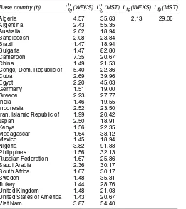
It is also important to compare the price indexes
gener-ated by the reliability measures 1/SjkP and 1/var(α˜jk)for both
the weighted-EKS and MST methods. These results along with EKS–Törnqvist (i.e., CCD) price indexes for 30 coun-tries are presented in Table 2, with the United States as the base. Again the full list for all 103 countries has been given by Hill and Timmer (2004). Particularly striking are the results for Cameroon; the price index differs by a factor of 9 depending on which method is used!
In the context of this article, we are particularly interested in
assessing the impact of the choice between using either 1/SPjk
or 1/var(α˜jk)as weights on the weighted-EKS and MST price
indexes. The following sensitivity measure is useful in this con-text:
wherezdenotes a weighted binary-based multilateral method
such as MST or weighted-EKS, f and g denote alternative
Table 1. Top 25 Bilateral Links in MST
Weighting scheme 1/SPjk Weighting scheme 1/var(αjk)
MST bilateral links 1/SPjk Njk MST bilateral links 1/var(αjk) Njk
Norway Niger 168.96 2 Slovakia Mexico 208.94 46 Norway Malaysia 75.16 2 Ireland Denmark 197.96 25 Sudan Canada 57.97 5 U.K. Ireland 188.76 30 Norway Albania 52.06 9 Zambia Tunisia 171.30 18 Norway New Zealand 48.62 12 Spain U.S.A. 159.91 75 Ireland Denmark 46.38 25 Norway Niger 154.54 2 Canada U.S.A. 43.62 24 Senegal Romania 153.37 19 U.K. Ireland 41.58 30 South Africa Mexico 153.33 57 Finland Canada 39.26 13 Canada U.S.A. 150.70 24 Peru Norway 37.15 10 Peru China 149.58 48 Norway Indonesia 36.43 3 Spain Greece 149.53 67 Norway Costa Rica 34.10 4 Zambia South Africa 148.92 27 Spain Norway 30.60 13 South Africa China 143.76 53 Malaysia Canada 29.43 4 Spain Portugal 140.12 55 Switzerland Malaysia 29.42 13 Morocco Jordan 139.84 37 Ireland Germany 29.13 29 Spain Italy 138.61 66 Norway Bangladesh 28.70 4 Zambia Saudi Arabia 133.84 10 Mali Georgia 27.88 4 Zambia Jordan 132.88 16 Portugal Norway 27.85 12 Zambia Guatemala 132.87 15 Slovenia Norway 27.81 13 Sweden Czech Rep 132.85 28 Ghana Canada 26.89 2 Sweden Malaysia 131.52 11 Tunisia Norway 26.43 9 Finland Canada 130.39 13 Mali Jordan 26.13 5 Italy Hungary 129.16 54 Sweden Canada 25.71 16 Slovakia Greece 127.77 47 Ukraine Sweden 25.61 15 Slovakia Brazil 127.68 32
weighting schemes such as 1/SPjk and 1/var(α˜jk),bdenotes the
base country, andPkf(z)/Pbf(z)denotes the price index for
coun-tryk obtained using methodz and weighting schemef, with
countryb as the base.Lbfg(z)can be interpreted as measuring
the average percentage impact on method z (with country b
as the base) of changing the weighting scheme from f tog,
or vice versa, becauseLbfg(z)=Lbgf(z). For example, the
mea-sured price indexes obtained using the MST method with the United States as the base differ on average by 20.7%
depend-ing on whether 1/SPjk or 1/var(α˜jk) is used as a weight. The
problem with this measure is that the results are not invariant to the choice of base country, as can be seen in Table 3. Indeed,
Lfgb(z)for z=MST and the weighting schemes f =1/SPjk and
g=1/var(α˜jk)ranges between 18.9% (when Japan is the base)
and 96.1% (when Guinea is the base). An overall measure of
the sensitivity of the price indexes of methodzto the choice of
weighting scheme is obtained by averaging the results forLbfg(z)
across all possible base countries,
Lfg(z)= 1
K
K
b=1
Lfgb(z).
The results,Lbfg(z), for 30 base countries are shown in Table 3
along with the overall average,Lfg(z), obtained from using all
103 countries in turn as the base. (Again, see Hill and Timmer 2004 for the complete results.) From Table 3, it is clear that the MST price indexes are more sensitive to the choice of weights than are the weighted-EKS price indexes. On average, the MST
price indexes change by 29.1%, depending on whether 1/SPjk
or 1/var(α˜jk)is used as a weight, whereas the weighted-EKS
price indexes change by only 2.1%. But even a 2.1% average change is quite significant. Hence for datasets containing many
gaps, the choice between 1/SPjk and 1/var(α˜jk)as a measure of
reliability can have a major impact on the resulting price in-dexes.
8. CONCLUSION
The latest round of the ICP is attempting to make detailed comparisons of price levels across almost all countries in the world (see Diewert 2004a; International Comparisons Program 2005). Even though the world comparison is being broken up into regional blocks, obtaining complete matrices of prices at basic heading level for all the countries in each regional block is a major undertaking that may result in either excessive ag-gregation of data or loss of characteristicity (i.e., countries may be forced to supply price data on products that are not repre-sentative of their consumption patterns). This problem arises frequently in international comparisons. Thus it may be coun-terproductive to try and eliminate all gaps. We have shown here that gaps (i.e., missing observations) in the data are not an insur-mountable problem, particularly when weighted binary-based multilateral methods are used. However, it is important that ex-plicit account be taken of these gaps when deciding how much weight is given to each bilateral comparison in the overall mul-tilateral comparison. Failure to make such an adjustment may compromise weighted binary-based methods precisely when they are most needed (i.e., in a comparison over a heteroge-neous set of countries). We have developed a method with strong theoretical foundations that automatically makes such an adjustment. Our weights, which are derived from the standard errors on Törnqvist price indexes, naturally penalize bilateral comparisons containing many gaps.
Our standard errors can also be modified for use in consumer datasets below the basic heading level (where no value shares are available). If countries identify products as representative or
Table 2. PPP Exchange Rates per U.S. Dollar for Agricultural Output
MST MST WEKS WEKS
SjkP var(αjk) SjkP var(αjk) EKS max/min
Algeria 65.1 54.1 61.9 59.1 61.2 1.20 Argentina 1.1 .8 1.0 1.0 1.0 1.39 Australia 1.3 1.3 1.4 1.4 1.4 1.14 Bangladesh 32.3 40.3 38.8 39.4 37.6 1.25 Brazil .9 .9 .9 .9 .9 1.08 Bulgaria 7.2 14.1 13.1 13.2 13.4 1.95 Cameroon 488.5 488.5 2,375.8 2,209.5 4,446.5 9.10 China 4.1 4.9 5.0 5.0 4.9 1.22 Congo, Dem. Republic of 1,435.0 1,744.6 1,931.1 2,031.3 3,368.7 2.35 Cuba 3.2 2.6 2.6 2.5 6.1 2.47 Egypt 3.7 2.9 3.4 3.3 3.3 1.30 Germany 2.2 2.3 2.3 2.3 2.2 1.05 Greece 329.3 430.0 462.0 470.1 471.9 1.43 India 17.5 19.7 19.6 19.5 19.3 1.13 Indonesia 2,116.8 2,624.8 2,663.7 2,719.5 2,623.1 1.28 Iran, Islamic Republic of 1,130.7 1,138.1 1,400.4 1,378.9 1,449.7 1.28 Japan 501.4 533.5 590.8 577.5 610.5 1.22 Kenya 24.2 29.4 33.2 33.4 33.1 1.38 Madagascar 1,549.2 1,259.7 1,360.9 1,348.2 1,304.7 1.23 Mexico 4.3 4.6 4.6 4.6 4.4 1.06 Nigeria 20.7 42.2 43.8 45.4 43.9 2.20 Philippines 22.8 31.1 35.7 35.9 34.9 1.58 Russian Federation 5.4 6.9 7.6 7.5 7.8 1.43 Saudi Arabia 15.2 13.3 15.2 14.9 15.5 1.17 South Africa 4.8 4.2 4.3 4.3 4.3 1.14 Sweden 10.9 9.1 10.8 10.7 10.7 1.20 Turkey 46,510.3 61,390.1 66,295.0 66,140.0 66,221.0 1.43 United Kingdom 1.0 1.0 .9 .9 .9 1.04 United States of America 1.0 1.0 1.0 1.0 1.0 1.00 Viet Nam 18,636.1 30,417.0 22,198.0 21,364.0 16,180.0 1.88 Finland 11.4 11.4 11.4 11.3 11.2 1.01 France 8.8 8.8 9.4 9.5 9.6 1.10 Georgia 3.0 4.7 6.0 6.1 6.5 2.19 Ghana 247.7 278.3 341.1 337.6 330.7 1.38 Guatemala 6.2 5.4 5.7 5.7 5.6 1.14 Guinea 580.5 1,213.1 1,124.4 1,155.8 1,087.1 2.09 Haiti 11.8 19.2 20.2 20.4 20.0 1.74 Honduras 5.6 6.5 7.3 7.1 7.1 1.29 Hungary 75.6 82.5 87.2 86.5 85.7 1.15 Iraq 1,029.0 793.2 953.7 907.6 941.4 1.30 Ireland .9 .9 .9 .9 .9 1.02 Israel 3.4 4.0 3.8 3.8 3.8 1.17 Italy 1,908.4 2,360.9 2,583.0 2,567.8 2,570.2 1.35 Jordan .7 .9 .9 .9 .9 1.25 Korea, Republic of 1,698.9 2,394.7 2,652.6 2,638.4 2,632.6 1.56 Latvia .3 .4 .4 .5 .4 1.51 Malawi 5.3 5.6 7.1 7.1 7.2 1.35 Malaysia 3.1 2.9 3.7 3.7 3.6 1.27 Mali 177.0 213.3 307.5 308.4 320.6 1.81 Morocco 14.1 13.2 15.4 15.2 15.5 1.17 Mozambique 980.6 920.2 1,059.5 1,055.0 1,029.0 1.15 Myanmar 71.6 77.6 66.9 67.6 64.9 1.19 Nepal 20.6 25.5 21.5 21.1 21.7 1.24 Netherlands 4.0 4.0 3.9 4.1 4.1 1.04 New Zealand 1.1 1.6 1.6 1.6 1.6 1.46 Nicaragua 6.2 6.2 9.2 9.2 10.0 1.61 Niger 566.0 701.9 708.3 692.8 692.1 1.25 Norway 13.9 17.2 17.4 17.6 17.5 1.27 Pakistan 14.0 18.8 18.2 18.3 18.6 1.34 Panama 1.6 1.7 1.7 1.7 1.7 1.07 Papua New Guinea 3.2 2.6 3.0 3.0 3.0 1.26 Paraguay 1,633.1 1,913.1 1,682.6 1,669.4 1,643.0 1.17 Peru 1.8 2.2 2.3 2.3 2.2 1.25 Poland 1.1 1.7 2.0 1.9 1.9 1.79 Portugal 185.6 236.2 246.0 247.1 248.7 1.34 Romania 1,438.7 1,151.9 1,206.5 1,209.3 1,209.2 1.25 Rwanda 358.5 378.9 398.7 389.8 385.1 1.11 Senegal 556.9 445.9 475.6 471.1 464.2 1.25 Slovakia 23.2 24.5 26.2 26.2 25.9 1.13 Slovenia 106.9 159.0 153.0 155.9 151.9 1.49 Spain 140.9 189.9 199.0 201.0 204.2 1.45
Continues
Table 2. (Continued.)
MST MST WEKS WEKS
SjkP var(αjk) SjkP var(αjk) EKS max/min
Sri Lanka 42.3 44.8 45.7 46.3 46.1 1.10 Sudan 192.6 192.6 227.7 226.0 225.8 1.18 Switzerland 3.8 4.6 4.4 4.5 4.5 1.22 Syrian Arab Republic 21.7 25.9 33.6 32.9 33.7 1.55 Tanzania, United Republic of 392.9 282.2 347.7 342.2 338.5 1.39 Thailand 26.1 27.6 26.8 27.1 26.0 1.06 Tunisia 1.1 1.2 1.2 1.2 1.2 1.14 Uganda 3,413.7 2,996.0 3,148.4 2,980.8 2,809.5 1.22 Ukraine 2.4 2.0 2.4 2.4 2.5 1.22 Uruguay 4.1 5.4 5.3 5.4 5.4 1.32 Venezuela, Boliv Republic of 192.3 210.1 212.9 212.7 209.1 1.11 Yemen 105.7 111.7 118.3 118.9 117.4 1.13 Zambia 73.0 64.1 63.9 64.4 62.9 1.16 Zimbabwe 2.1 2.4 3.7 3.7 3.7 1.75
unrepresentative, these representative or unrepresentative iden-tifiers can be used to construct proxy value shares (i.e., each representative product is allocated an equal share, and unrep-resentative products are allocated a zero share), thus allowing computation of our standard errors. This means that weighted binary-based multilateral methods can be applied even below basic heading level.
In the process of developing our method, we have also forged new links between the stochastic and axiomatic approaches to index numbers. In particular, we have shown that one of Diewert’s relative price dissimilarity measures (derived in an axiomatic setting) is a special case of our preferred measure (derived in a stochastic setting).
Table 3. Sensitivity of the Multilateral Price Indexes to the Choice of Weighting Scheme [f=1/SP, g=1/var(α)]
Base country (b) Lbfg(WEKS) Lbfg(MST) Lfg(WEKS) Lfg(MST)
Algeria 4.57 35.63 2.13 29.06 Argentina 2.43 55.35
Australia 2.02 18.94 Bangladesh 2.08 23.84 Brazil 1.47 18.94 Bulgaria 1.47 82.80 Cameroon 7.35 20.67 China 1.49 21.53 Congo, Dem. Republic of 5.40 22.36 Cuba 2.69 39.96 Egypt 2.20 45.03 Germany 1.51 19.00 Greece 2.23 27.77 India 1.46 19.55 Indonesia 2.52 23.50 Iran, Islamic Republic of 1.99 20.42 Japan 2.50 18.91 Kenya 1.56 22.35 Madagascar 1.64 38.12 Mexico 1.45 18.94 Nigeria 3.82 91.88 Philippines 1.56 32.13 Russian Federation 1.67 25.86 Saudi Arabia 2.36 30.17 South Africa 1.67 30.17 Sweden 1.48 35.31 Turkey 1.44 28.76 United Kingdom 1.48 21.03 United States of America 1.43 20.67 Viet Nam 3.87 54.40
ACKNOWLEDGMENTS
The authors thank participants at the University of California Davis Workshop on Estimating Production and Income Across Nations, April 13–14, 2004 (particularly Erwin Diewert) for helpful comments.
[Received November 2004. Revised September 2005.]
REFERENCES
Allen, R. C., and Diewert, W. E. (1981), “Direct versus Implicit Superlative Index Number Formulae,”Review of Economics and Statistics, 63, 430–435. Balk, B. M. (1996), “A Comparison of Ten Methods for Multilateral Inter-national Price and Volume Comparison,”Journal of Official Statistics, 12, 199–222.
Caves, D. W., Christensen, L. R., and Diewert, W. E. (1982), “Multilateral Com-parisons of Output, Input and Productivity Using Superlative Index Num-bers,”The Economic Journal, 92, 73–86.
Clements, K. W., and Izan, H. Y. (1981), “A Note on Estimating Divisia Index Numbers,”International Economic Review, 22, 745–747.
Cuthbert, J. R. (2000), “Theoretical and Practical Issues in Purchasing Power Parities Illustrated With Reference to the 1993 Organization for Economic Cooperation and Development Data,”Journal of the Royal Statistical Soci-ety, Ser. A, 163, 421–444.
Cuthbert, J. R., and Cuthbert, M. (1989), “On Aggregation Methods for Pur-chasing Power Parities,” Working Paper No. 56, Dept. of Economics and Statistics, OECD, Paris.
Diewert, W. E. (1976), “Exact and Superlative Index Numbers,”Journal of Econometrics, 4, 115–145.
(1995), “On the Stochastic Approach to Index Numbers,” Discussion Paper 95-31, University of British Columbia, Dept. of Economics.
(1999), “Axiomatic and Economic Approaches to International Com-parisons,” inInternational and Interarea Comparisons of Income, Output and Prices, eds. A. Heston and R. E. Lipsey, Chicago: NBER, University of Chicago Press, pp. 13–87.
(2001), “The Consumer Price Index and Index Number Theory: A Sur-vey,” Discussion Paper 01-02, University of British Columbia, Dept. of Eco-nomics.
(2002), “Similarity and Dissimilarity Indexes: An Axiomatic Ap-proach,” Discussion Paper 02-10, University of British Columbia, Dept. of Economics.
(2004a), “On the Stochastic Approach to Linking the Regions in the ICP,” Discussion Paper 04-16, University of British Columbia, Dept. of Eco-nomics.
(2004b), “Elementary Indices,” inConsumer Price Index Manual: Theory and Practice, Geneva: International Labour Organization, pp.??–??. Eltetö, O., and Köves, P. (1964), “On a Problem of Index Number Computation
Relating to International Comparison,”Statisztikai Szemle, 42, 507–518. Geary, R. G. (1958), “A Note on the Comparison of Exchange Rates and PPPs
Between Countries,”Journal of the Royal Statistical Society, Ser. A, 121, 97–99.
Gini, C. (1931), “On the Circular Test of Index Numbers,”International Review of Statistics, 9, 3–25.
Hicks, J. R. (1946),Value and Capital(2nd ed.), Oxford, U.K.: Clarendon Press.
Hill, R. J. (1997), “A Taxonomy of Multilateral Methods for Making Interna-tional Comparisons of Prices and Quantities,”Review of Income and Wealth, 43, 49–69.
(1999), “Comparing Price Levels Across Countries Using Minimum Spanning Trees,”Review of Economics and Statistics, 81, 135–142.
(2004), “Constructing Price Indexes Across Countries and Time: The Case of the European Union,”American Economic Review, 94, 1379–1410. Hill, R. J., and Timmer, M. P. (2004), “Standard Errors as Weights in
Mul-tilateral Price Indexes,” GGDC Working Paper GD-200473, University of Groningen.
Iklé, D. M. (1972), “A New Approach to the Index Number Problem,”Quarterly Journal of Economics, 86, 188–211.
International Comparisons Program (2005), Handbook, Washington, DC: World Bank.
Khamis, S. H. (1972), “A New System of Index Numbers for National and International Purposes,”Journal of the Royal Statistical Society, Ser. A, 135, 96–121.
Leontief, W. (1936), “Composite Commodities and the Problem of Index Num-bers,”Econometrica, 4, 39–59.
Rao, D. S. P. (1999), “Weighted EKS Method for Aggregation Below Basic Heading Level Accounting for Representative Commodities,” short note pre-pared for the ICP Unit, OECD.
(2001), “Weighted EKS and Generalized CPD Methods for Aggrega-tion at Basic Heading Level and Above Basic Heading Level,” presented at the Joint World Bank–OECD Seminar on Purchasing Power Parities, Wash-ington, DC, January 30–February 2, 2001.
Rao, D. S. P., and Timmer, M. (2003), “Purchasing Power Parities for Industry Comparisons Using Weighted Eltetö–Köves–Szulc (EKS) Methods,”Review of Income and Wealth, 49, 491–511.
Rao, D. S. P., Ypma, G., and van Ark, B. (2003), “Agricultural Purchasing Power Parities and International Comparisons of Agricultural Output and Productivity,” mimeo, Groningen Growth and Development Centre. Selvanathan, E. A., and Rao, D. S. P. (1994),Index Numbers: A Stochastic
Approach, Ann Arbor, MI: University of Michigan Press.
Summers, R., and Heston, A. (1991), “The Penn World Table (Mark 5): An Ex-panded Set of International Comparisons, 1950–1988,”Quarterly Journal of Economics, 106, 327–368.
Szulc, B. (1964), “Indices for Multiregional Comparisons,”Przeglad Statysty-czny, 3,Statistical Review, 3, 239–254.
van Veelen, M. (2002), “An Impossibility Theorem Concerning Multilateral International Comparison of Volumes,”Econometrica, 70, 369–375. Wilson, R. J. (1985), Introduction to Graph Theory(3rd ed.), New York:
Longman.