Full Terms & Conditions of access and use can be found at
http://www.tandfonline.com/action/journalInformation?journalCode=ubes20
Download by: [Universitas Maritim Raja Ali Haji] Date: 13 January 2016, At: 00:38
Journal of Business & Economic Statistics
ISSN: 0735-0015 (Print) 1537-2707 (Online) Journal homepage: http://www.tandfonline.com/loi/ubes20
Testing the Normality Assumption in the Sample
Selection Model With an Application to Travel
Demand
Bas van der Klaauw & Ruud H Koning
To cite this article: Bas van der Klaauw & Ruud H Koning (2003) Testing the Normality Assumption in the Sample Selection Model With an Application to Travel Demand, Journal of Business & Economic Statistics, 21:1, 31-42, DOI: 10.1198/073500102288618739
To link to this article: http://dx.doi.org/10.1198/073500102288618739
Published online: 01 Jan 2012.
Submit your article to this journal
Article views: 58
View related articles
Testing the Normality Assumption in the
Sample Selection Model With an
Application to Travel Demand
Bas
van der Klaauw
Department of Economics, Free University Amsterdam, De Boelelaan 1105, NL-1081 HV Amsterdam,
The Netherlands and Scholar (klaauw@tinbergen.nl)
Ruud H. K
oning
Department of Econometrics, University of Groningen, P.O. Box 800, NL-9700 AV Groningen,
The Netherlands (r.h.koning@eco.rug.nl)
In this article we introduce a test for the normality assumption in the sample selection model. The test is based on a exible parametric specication of the density function of the error terms in the model. This specication follows a Hermite series with bivariate normality as a special case. All parameters of the model are estimated both under normality and under the more general exible parametric specication, which enables testing for normality using a standard likelihood ratio test. If normality is rejected, then the exible parametric specication provides consistent parameter estimates. The test has reasonable power, as is shown by a simulation study. The test also detects some types of ignored heteroscedasticity. Finally, we apply the exible specication of the density to a travel demand model and test for normality in this model.
KEY WORDS: Flexible parametric density estimation; Hermite series; Heteroscedasticity; Sample selection.
1. INTRODUCTION
Maximum likelihood is the most popular estimation method in microeconometrics. The method yields consistent (in fact, asymptotically efcient) estimators if the model is specied correctly. However, correct specication may not be known beforehand. Two major sources of misspecication are incor-rect specication of the functional form of the relationship under study (e.g., omitting exogenous variables or inappropri-ately assuming linearity) and misspecication of the stochastic structure of the model (e.g., neglecting heteroscedasticity or misspecication of the distribution of the random variables). The maximum likelihood estimator is generally inconsistent in these cases. This is particularly true in the case of limited dependent variable models (e.g., Hurd 1979; Smith 1989). In this article we focus on one particular form of misspecica-tion: misspecication of the distribution of the error terms. We retain the assumption of correct specication of the functional form of the relationship.
The model that we study is the sample selection model introduced by Heckman (1979). This type of model accounts for problems arising because the outcome of the endogenous variable is observed only for a (selective) part of the sam-ple. For example, sample selection models are used to study wage equations, where only the wages of employed workers are observed (e.g., Buchinsky 1998; Melenberg and Van Soest 1993). This model is not only very useful when the outcome variable is only observed for a (nonrandom) part of the popu-lation, but it can easily be extended to the switching regression model. The switching regression model is the point of depar-ture for many interesting problems in economics. For exam-ple, it is used to evaluate active labor market programs (Heck-man, LaLonde, and Smith 1999), to investigate the effect of
migration on earnings (Tunalõ 2000), to study the returns to
eduction (Heckman, Tobias, and Vytlacil 2000), and to esti-mate the effect of union membership on earnings (Lee 1978). In the switching regression model, many of the interesting policy parameters, such as the treatment effect on the treated, depend not only on the functional form of the relationship, but also on the joint distribution of the error terms. Therefore, for policy evaluation and also for simulations, both the parameters of the functional form of the relationship and the joint distri-bution of the error terms must be known. Of course, this does not hold for either the switching regression model, or also for other models, like the sample selection model.
Usually, the sample selection model is estimated either by maximum likelihood or by Heckman’s two-step procedure (Heckman 1979), under the assumption that the error term in the regression equation and the error term in the selection equation follow a bivariate normal distribution. However, it is often argued that the parameter estimates are sensitive to the distributional assumptions (Manski 1989). In fact, Newey (1999a) proved that only under very restrictive assumptions, the parameter estimates are consistent against misspecication of the distribution of the error terms. In many cases, the nor-mal distribution might be overly restrictive. As mentioned ear-lier, the sample selection model is often used to model earn-ings, and it is well known from the economic literature that the distribution of (the logarithm of) earnings in the popula-tion has fatter tails than the normal distribupopula-tion funcpopula-tion (e.g., Heckman et al. 2000).
©2003 American Statistical Association Journal of Business & Economic Statistics January 2003, Vol. 21, No. 1 DOI 10.1198/073500102288618739
31
We introduce a formal test for the normality assumption within the sample selection model. The test is motivated by the seminonparametric maximum likelihood estimation method of Gallant and Nychka (1987) in which the true distribution of the error terms is approximated by a Hermite series. The density of the error terms follows a very exible parametric specication, which is estimated using maximum likelihood together with all other parameters of the model. The test thus provides an alternative distribution of the error terms in the event that normality is rejected. Because the parameters are estimated using maximum likelihood, the estimators are
ef-cient, pN consistent, and asymptotically normal. To
exam-ine the power of the normality test, we perform a simulation study, which will also provide practical experience about the actual exibility of the parametric specication of the den-sity. For the binary choice model and duration models, Smith (1989) proposed a similar type of polynomial specication to test for normality. Gabler, Laisney, and Lechner (1993) pro-vided Monte Carlo evidence on this test and applied it to a model of female labor force participation.
So far we did not discuss heteroscedasticity of the error terms. Ignored heteroscedasticity causes the usual estima-tors in limited dependent-variable models to be inconsistent. For example, Hurd (1979) showed that the bias caused by ignored heteroscedasticity is severe in the truncated regres-sion model. Not many estimation procedures are robust against heteroscedasticity. An exception is the quantile regression approach of Buchinsky (1998). The disadvantage of quantile regression methods is that the complete distribution of the error terms is not estimated. This complicates performing sim-ulations, and because the mean is not estimated, it is difcult to dene relevant policy parameters (see Abadie, Angrist, and Imbens 1998, who applied the quantile regression estimator to the switching regression model). In our simulation study we also focus on the robustness of the exible parametric density against heteroscedastic error terms.
An advantage of the exible parametric density used in this article is its general applicability; it is not specic to one par-ticular econometric model. The approach taken herein can be used to examine the sensitivity of estimation results to the assumption of normality in other microeconometric models where no formal test of normality is available. We illustrate both the exible parametric density and the normality test in a model of travel demand and car ownership.
The article is organized as follows. Section 2 discusses the sample selection model and the exible parametric density that naturally leads to a normality test for the sample selection model. Section 3 reports some simulations to investigate the performance of the exible parametric density and the power of the normality test. Section 4 discusses an application of the estimation method and the normality test to the model of travel demand. Finally, Section 5 concludes.
2. IDENTIFICATION AND ESTIMATION OF THE
SAMPLE SELECTION MODEL
In this section we discuss some identication and estima-tion issues associated with the sample selecestima-tion model. In par-ticular, we focus on the exible parametric density that leads to a test for bivariate normality.
Within a population, we are interested in the distribution
of an outcome variable y conditional on a vector of
exoge-nous variablesx1. Therefore, we specify for individuali 4iD
11 : : : 1 N 5the regression equation
yiD‚0
1x1iC˜1i0 (1)
The dependent variableyiis observed for a subsample only. A
binary variablezi is introduced that equals 1 if the realization
of yi is observed and otherwise equals 0. The selection rule
depends on a set of exogenous variablesx2and is given by
züi D‚02x2iC˜2i
As mentioned in Section 1, we focus only on the joint distri-bution of the error terms4˜1i1 ˜2i5, and thus we simply assume
linear specications in both the regression and the selection equation. If the conditional expectation of ˜1i given ziD1
does not equal 0, ordinary least squares (OLS) estimation of (1) will not yield consistent estimates for the parameters of interest,‚1.
If one is willing to assume that the error terms4˜1i1 ˜2i5
fol-low a bivariate normal distribution, then the model can be esti-mated using Heckman’s two-stage procedure (see Heckman 1979). In the rst step, a probit model is estimated for the selection equation to obtain‚O2, in the second step, the
regres-sion equation
yiD‚01x1iC‘1
”4‚O20x2i5
ê4‚O20x2i5C‡i (3)
is estimated (by OLS) for the subsample for which a real-ization of yi is actually observed 4ziD15. The parameter
denotes the correlation between ˜1 and ˜2, and ‘
2 1 is the
variance of ˜1 (the variance of ˜2 is normalized to 1). If
the vectorx1i equals the vectorx2i, then identication of the
model hinges entirely on the functional form and distributional assumptions, which makes the parameter estimates very sen-sitive to the distributional assumptions (see Manski 1989 for an extensive overview). Therefore, in most economic applica-tions, an exclusion restriction is imposed—at least one vari-able enters only the selection equation and not the regression equation.
The bivariate normality assumption may be overly restric-tive. Therefore, starting with Lee (1982), who modied Heck-man’s two-step procedure to allow in a general way for departures from normality, a number of estimation methods have been introduced that relax the distributional assump-tions. These (semiparametric) estimation methods general-ize the probit estimation in the rst step to, for example, kernel-based estimation and use more exible error correc-tion terms in the regression equacorrec-tion (e.g., Ahn and Powell 1993; Cosslett 1991; Ichimura and Lee 1991; Newey 1999b). This provides consistent estimators for the parameters of
inter-est ‚1, but computation of the corrected standard errors of
these parameters is quite cumbersome (e.g., Ahn and Powell
1993; Cosslet 1991). A main disadvantage of most semipara-metric estimation methods is that the intercept in the outcome equation remains unidentied (and thus cannot be estimated). As stressed by Heckman (1990), in many economic applica-tions the intercept is an important parameter of interest.
The alternative to two-step estimation is maximum likeli-hood estimation. This requires full specication of the joint density function of the error terms, which is denoted by
f 4˜11 ˜25. Under the assumption of correct specication,
max-imum likelihood estimation yields consistent estimates of all parameters of interest and straightforward computation of the asymptotic distribution. The log-likelihood function of the sample selection model is
In maximum likelihood estimation, consistency depends crucially on the correct specication of the joint density of the error terms. Therefore, it is convenient to specify this density so that it is exible. We use exible parametric specications that are inspired by seminonparametric estimation as intro-duced by Gallant and Nychka (1987). The unknown density functionf 4˜11 ˜25is approximated by a Hermite series.
We consider densitiesh4˜5in a subclass¨K that are of the
Hermite form
normal density function with mean 0 and covariance matrixè.
In fact, Gallant and Nychka (1987) restricted è to being a
diagonal matrix. Because of the squaring, no restrictions are necessary to ensure thathü4˜5is nonnegative. Some restric-tions are required to ensure that the density integrates to 1 and for identication. We return to these restrictions later.
Gallant and Nychka (1987) showed that a large class ¨
of density functions can be approximated arbitrarily well by
increasing the number of terms K of the polynomialPK4˜5.
They gave the precise conditions dening ¨. For our
pur-poses, it sufces to note that the fattest tails allowed aret-like tails, and the thinnest tails allowed are thinner than normal-like tails. Any sort of skewness and kurtosis (especially in that part of the distribution where most probability mass is observed) is allowed, and only very violently oscillatory densities are
excluded from¨. Gallant and Nychka (1987) proved that the
densities in¨ can be estimated consistently by increasingK
with the number of observations. In (5), the normal density is used as the base class for ¨K, but this is not necessary; any density with a moment-generating function could be used (see, e.g., Cameron and Johansson 1997).
It is also possible to assume that the true density is a
mem-ber of ¨K and hence to interpret ¨K as a exible class
of density functions. This is the interpretation that we fol-low in this article. This interpretation is especially appealing if one wants to examine the sensitivity of estimation results
obtained by assuming normality to this distributional assump-tion, because it allows one to use the standard framework of inference. Because we want to test for bivariate normality (with unrestricted correlation) in the sample selection model, we do not restrict the covariance matrix, unlike Gallant and Nychka (1987). This provides a formal test for normality in the sample selection model; that is, PK4˜5 is constant for all values of˜. Such a test for normality has not yet been derived in the literature. An alternative could be to perform Hausman tests on the slope coefcients of the regressions equation. One could either use Hausman tests to test normality against a semiparametric alternative or also against the exible para-metric alternative discussed in this article. The rst alternative may be somewhat cumbersome, because it requires comput-ing standard errors in the semiparametric estimation, which is not always straightforward. The second alternative is easy to implement, but these tests are not expected to be as powerful as the tests derived in this article. The simulations in Section 3 indicate that the slope coefcients are not very sensitive to departures from normality. Hausman tests leave out any infor-mation on the distribution of the error terms.
In line with Gallant and Nychka (1987), we parameterize
hü4˜5as
This bivariate density can be easily generalized to a den-sity function for more variables, which is important when, for example, studying switching regression models containing three error terms. To ensure that this density integrates to 1, a restriction on the parameters is necessary. This restriction can take the form of an explicit restriction on the parameters of the density. However, for computational convenience, we follow Gabler et al. (1993), who ensured integration to 1 by
scaling the density. DeneS by
SDZ
Because of the denition ofS, the following density integrates to 1:
h4˜5Dhü4˜5=S0
It is clear that the parameters are identied up to a scale
only, so normalization is necessary. Therefore, we impose
00D1. ForKD0,h4˜5now reduces to the bivariate normal
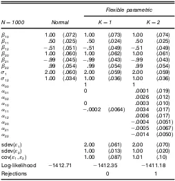
density. The exibility of this family of densities is illustrated in Figures 1–3 (KD2). It is clear that the contour lines differ from the usual ellipsoids of the bivariate normal density.
In the sample selection model, identication is achieved by settingè22D
p
2, to ensure identication of the scale of (2). To x the location of the distribution function, we optimize the log-likelihood function (4) under the restrictions that the
Figure 1. Bivariate Flexible Parametric Density,01D.1,
10D-.1, and11D-.2.
means of˜1 and˜2equal 0. Alternatively, one could impose
explicit restrictions on the parameters to ensure that the
means of˜1and˜2are 0. However, forK¶2, these are rather
complex nonlinear restrictions. Another alternative was pro-posed by Melenberg and Van Soest (1993), who suggested not imposing restrictions on the parameters of the density function of˜to ensure a zero mean, but rather restricting the intercepts of (1) and (2). For the purpose of this article, such a strategy is not very useful. Our approach allows testing the null hypoth-esis that4˜11 ˜25 is distributed according to a normal
distri-bution function against the alternative hypothesis that4˜11 ˜25
has some other mean zero bivariate distribution function in the
class of distribution functions¨K for any xedK. In other
words, for some xedK, we test for joint signicance of all
ij withiCj¶1. The additional number of parameters under the alternative hypotheses compared to the null hypotheses is4KC152ƒ1. Note that there are two restrictions on these
parameters to x the location of the distribution. Therefore,
Figure 2. Bivariate Flexible Parametric Density,01D.1,
10D.1, and11D0.
the likelihood ratio test statistic is distributed according to a chi-squared distribution with4KC152ƒ3 degrees of freedom.
Optimizing the log-likelihood function subject to the means of˜1 and˜2 being equal to 0 requires evaluating the relevant
integrals in the log-likelihood function and the expressions for the means. Because of the general covariance matrix in the
base function ”4˜—è5, these integrals do not have the same
computationally attractive properties as they do when using the base function proposed by Gallant and Nychka (1987). However, because of the special structure of the sample selec-tion model, we are able to avoid evaluaselec-tions of bivariate nor-mal integrals, so the computational cost of this generalization is limited. Appendix A gives the recursion formulas that can be used to determine the relevant integrals explicitly.
Finally, the exible parametric density discussed earlier assumes homoscedasticity of the error terms. As is clear from (3), the estimators are not robust against ignored heteroscedas-ticity (i.e., ‘1 is not the same for all observations). In the
Figure 3. Bivariate Flexible Parametric Density,01D.1,
10D-.1, and11D.2.
next section we also discuss the performance of the exible parametric density in case the error terms are heteroscedas-tic. In particular, we focus on heteroscedasticity in ˜1 when
the correlationbetween˜1 and˜2 is constant. Note that the
variance of ˜2 is generally unidentied. Thus many types of
heteroscedasticity in the distribution of˜2could be solved by
generalizing the single index in (2).
3. SIMULATION STUDY
In this section we perform a limited simulation exercise to investigate the performance of the exible parametric density and the power of the normality test discussed in Section 2. We focus two main sources of inconsistency, departures from normality and heteroscedasticity in the error terms.
We consider the simulation experiment
yiD‚10C‚11xiC‚12wiC˜1i
and
züi D‚20C‚21viC‚22wiC˜2i1 iD11 : : : 1 N 1
with true parameters ‚10D1, ‚11D05, ‚12 D ƒ05, ‚20 D1,
‚21D ƒ1, and ‚22 D1. The exogenous variablesxi and vi
are independently®40135 distributed, and wi is distributed uniformly on 6ƒ3137. We perform ve experiments in which
we vary the distribution of ˜. The sample size N is 1000.
(Similar simulation experiments with a sample size N equal
to 500 gave the same results and are available on request.) Within each experiment, we draw 100 samples. In the rst
three experiments, we draw ˜ from either a bivariate
nor-mal distribution with mean 0, a bivariate t distribution, or
a centered chi-squared distribution. The t distribution has
fatter tails than the normal distribution and the chi-squared distribution is asymmetric, so both these cases are a devia-tion from normality. For all experiments, we set var4˜15D4,
var4˜25D1, and cov4˜11 ˜25D1. In the last two
experi-ments, the error terms are bivariate normal distributed but
heteroscedastic. First, the distribution of ˜ depends on the
explanatory variable x. Second, we distinguish three groups
of individuals who have different covariance matrices. (This simulation experiment has some similarities with experiments in Hurd 1979.) The details of the simulation experiments are given in Appendix B. The simulations were performed on Pen-tium workstations using the constrained maximum likelihood (CML) library of GAUSS.
Because the computer time required for optimization of the log-likelihood function increases quickly withK, we estimate
only the model for KD1 and KD2 and for the bivariate
normal distributed disturbances. Hence we consider the nor-mality test against the class of exible parametric densities
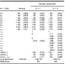
Table 1. Results of the Simulation Experiment With Bivariate Normal Distributed Disturbances
Flexible parametric
ND1000 Normal KD1 KD2
‚10 1000 (0072) 1000 (0073) 1000 (0074) ‚11 050 (0025) 050 (0024) 050 (0025) ‚12 ƒ051 (0051) ƒ051 (0049) ƒ051 (0049) ‚20 1000 (0060) 1000 (0062) 1000 (0061) ‚21 ƒ099 (0045) ƒ099 (0043) ƒ099 (0043) ‚22 099 (0054) 099 (0054) 099 (0054) ‘1 2000 (0060) 2000 (0059) 2000 (0059) ‘12 1000 (0034) 1000 (0036) 1000 (0036)
00 1 1
01 0 00001 (0019) 02 00026 (0012) 10 0 00003 (0010) 11 ƒ00002 (00064) 00034 (0017) 12 00006 (0017) 20 ƒ00004 (00051) 21 ƒ00005 (00067) 22 ƒ00014 (00050)
sdev(˜1) 2000 (0061) 2000 (0070)
sdev(˜2) 1000 (0013) 1000 (0020)
cov(˜11 ˜2) 1000 (0087) 1001 (010)
Log-likelihood ƒ1412.71 ƒ1412.35 ƒ1411.18
Rejections 0 1
NOTE: Standard errors are given in parentheses.
Table 2. Results of the Simulation Experiment With Bivariate t
Log-likelihood ƒ1371.30 ƒ1348.14 ƒ1331.18
Rejections 69 97
NOTE: Standard errors are given in parentheses.
withKD1 and KD2 (denoted by ¨ü
1 and ¨2ü). The case
of the normal disturbances is presented in detail in Table 1; the case of thetdisturbances, in Table 2; and the case of the chi-squared disturbances, in Table 3. The simulation results from the heteroscedastic error terms are presented in Table 4 for the covariance matrix dependent on the observed variable
Table 3. Results of the Simulation Experiment With Bivariate Chi-Squared Distributed Disturbances
Log-likelihood ƒ1403.24 ƒ1391.81 ƒ1345.13
Rejections 89 100
NOTE: Standard errors are given in parentheses.
Table 4. Results of the Simulation Experiment, Where the Error Terms are Distributed According to a Bivariate Normal Distribution With
Heteroscedasticity Depending on the Explanatory Variablex
Flexible parametric
Log-likelihood ƒ1436.58 ƒ1362.86 ƒ1315.80
Rejections 100 100
NOTE: Standard errors are given in parentheses.
x and in Table 5 for the covariance matrix dependent on an
unobserved variable.
It is remarkable how well standard maximum likelihood under the assumption of normally distributed disturbances per-forms. Departures from normality do not cause serious bias
Table 5. Results of the Simulation Experiment, Where the Error Terms are Distributed According to a Bivariate Normal Distribution With Heteroscedasticity Depending on an Unobserved VariablerTaking
Three Possible Values,p.5, 1, and p
Log-likelihood ƒ1405.10 ƒ1405.09 ƒ1402.10
Rejections 0 12
NOTE: Standard errors are given in parentheses.
in the parameter estimates. In case the true disturbances
fol-low a t distribution, all estimated parameters are within two
standard deviations of their true values. This is the case even when the disturbances follow a transformed chi-squared dis-tribution that is nonsymmetric. This suggests that if obtain-ing estimates for the parameters‚ is the only interest, than it is sufcient to assume normality and obtain estimates. How-ever, in the presence of heteroscedasticity in the error terms that is dependent on one of the observed exogenous variables, the parameter estimates under normality are somewhat biased (see Table 4). In particular, the parameter estimate of‚11
dif-fers from the true value. This bias disappears when estimating the model using the exible parametric specication. When the heteroscedasticity does not depend on exogenous variables but the covariance matrix differs between groups, the parame-ter estimates obtained under normality are again close to their true value.
Tables 1–5 also report the number of rejections of normality for each simulation experiment. The simulation results indi-cate that the normality test against both the class¨ü
1 and¨2ü
performs well. The number of incorrect rejections is small when compared to the level of signicance. The number of correct rejections is very high except in the simulation experi-ment, where the distribution of the error terms differs between groups. The test is very powerful when the error terms are not bivariate normal distributed, and it is successful in detect-ing heteroscedasticity dependdetect-ing on observed exogenous vari-ables. The simulation results indicate that the test has more
power when the tted distribution belongs to¨ü
2 than when
it belongs to¨ü
1. Because departures from normality do not
cause serious bias in the parameter estimates of the regres-sion equation, Hausman tests for normality against a semi-parametric alternative probably will not be as powerful as the likelihood-based tests discussed in this article.
The results from the simulation study suggest that the
esti-mates for the ‚1 parameters (derived under the assumption
of normality) are reasonably robust to misspecication of the error term. This is not true only if the covariance matrix of the error terms depends on observed explanatory variables. In this case, using the exible parametric density can help improve the parameter estimates. Furthermore, if one is interested not
only in the parameter estimates of ‚1, but also in the
com-plete distribution function of outcome variabley conditional
on explanatory variablesx, then using the exible parametric specication is worthwhile.
4. AN APPLICATION TO A MODEL OF
TRAVEL DEMAND
In this section we apply the exible parametric estimation procedure and the normality tests to a model describing travel demand. This section consists of three parts: rst, we present a structural model, then we discuss the data, and nally, we present the empirical results.
The model assumes that in a given year households need to travel a stochastic number of kilometers and that these house-holds minimize the costs of traveling. At the beginning of the year, a household makes a prediction of the number of kilome-ters to be traveled, which is denoted byyü. The actual number
of kilometers traveled in this year is related to the prediction byyDyü
¢˜, where˜is a random prediction error with a
pos-itive support and a nite meanŒ. The household can choose
to travel either by car or by other means. The latter is most likely public transportation; other possibilities may be bikes, car pooling, and so forth. The cost of using a car consists of xed costs,cc, and variable costs, vc. Fixed costs are
depre-ciation of the car, maintenance, insurance, and taxes for car ownership. Variable costs are the costs of fuel. The costs of other transportation do not contain any xed costs. The
vari-able costs, denoted by vo, are associated with the costs of
public transportation. However, opportunity costs may also be important, because traveling with public transportation usually takes more time than traveling by car.
The household decision problem now involves choosing whether or not to use a car. Assuming that (risk-neutral) households minimize their expected costs, the decision rule implies that a car is used if
E6ccCvcy7µE6voy70 (6)
Now assume thatcc,vc, andvo are known by the household.
This means that the household decision simplies to using a car if
E6y7¶ cc
voƒvc0 (7)
If we substitute the relation between the actual number of kilometers driven and the predicted number of kilometers, then this implies that a household chooses to use a car if
yü¶ cc
Œ4voƒvc5
0
Now we parameterize the unknown components of the model as
yüDexp4x0‚Cv151
which is the distance function and a costs function
cc
voƒvc
Dexp4z0ƒCv251
wherev1andv2denote unobserved individual specic effects.
We normalizeŒD1.
The model reduces to a regression equation, which has the structure
log4y5Dx0‚C˜
1
with ˜1Dv1Cln4˜5. A selection equation indicates whether the household owns a car,
x0‚ƒz0ƒC˜
2¶01
with the household-specic term˜2equal tov1ƒv2, which is
known to the household but unknown to the econometrician. Becausev1 is included in both˜1 and˜2, these disturbances are not a priori independent.
To improve the identication of the model, we impose an exclusion restriction, that is, nd a variable that is included in
zand excluded fromx. According to the model, the predicted
number of kilometers affects both the actual number of kilo-meters and the decision to buy a car, whereas the xed and
variable costs of using a car and the variable costs of other transportation affect only the decision of whether to use a car. Thus the exclusion restriction should be a variable that affects only the costs functions. Because the Dutch government pro-vides free public transportation passes to some students and some civil servants, we use the dummy variable that indicates whether the household has such a free public transportation pass as a variable which is included inzbut not in x.
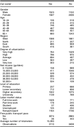
The data we use is a subset from the Dutch database on transportation behavior of Statistics Netherlands. This database contains 34,454 households. To avoid complica-tions of households owning more than one car, we focus on single-person households. Furthermore, we exclude individu-als younger than age 18 years, the legal age for obtaining a drivers license in The Netherlands. This restricts the database to 7404 individuals. To construct our nal dataset, we also exclude 130 individuals who own a car but for whom the num-ber of kilometers driven in the past year is unknown and also 756 individuals for whom one or more explanatory variables are missing. Our nal dataset consists of 6518 observations.
Table 6 provides some characteristics of the dataset. The data contain 3110 individuals who own a car and 3408 who do not own a car. Except for region, all variables display dif-ferences in car ownership rates. Although 58% of the men are car owners, only 41% of the women have a car. Until people reach age 65, the car ownership rate increases with age; after that, there is a large drop. Furthermore, car ownership rates increase with income and level of education. Finally, individ-uals living in areas with a low degree of urbanization, full-time employed workers, and individuals who do not have a government-provided free public transportation pass are more likely to own a car than their counterparts.
Using these data, we estimate the structural model discussed previously. In the rst step, we estimate the model under the assumption that the disturbances˜1 and˜2 follow a bivariate normal distribution. Next, we relax this assumption by assum-ing that the density of the disturbances belongs to either¨ü
1
or¨ü
2. For these two cases, we test whether the restriction of
normality of the disturbances can be imposed.
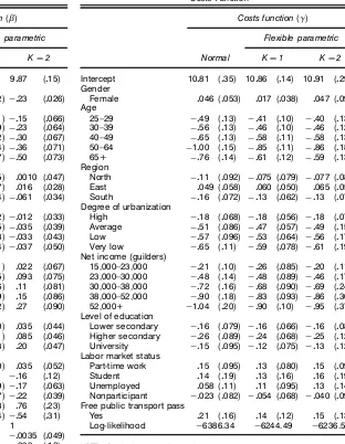
All parameter estimates are presented in Tables 7 and 8. The parameter estimates of the distance function (Table 7) and of the costs function (Table 8) are not very sensitive to the spec-ication of the distribution function of the error term, which is in line with the results from the simulation study. The most important covariates in the distance function are gender, age, income, level of education, and individual labor market status; those in the costs function are age, degree of urbanization, and income. Although the availability of a free public transporta-tion pass provided by the government has the expected effect on the costs function, the corresponding parameter estimate is not signicantly different from 0.
The only individual characteristics important in both the dis-tance and costs functions are age and income. Age affects both the distance function and the costs function negatively. Young people travel more kilometers than older people, whereas the costs of car use relative to other transportation modes decrease with age. By comparing the coefcients, we can see that per-sons age 50–64 are most likely to own a car. Income has an opposite effect on the distance and costs functions. Persons
Table 6. Some Characteristics of the Dataset
Car owner Yes No
Average number of kilometers 151093
Observations 3110 3408
with greater income travel more kilometers, whereas the costs of car use relative to other transportation decrease. Consider-ing that usConsider-ing public transportation takes more time, this latter effect can be explained by differences in opportunity costs. Time is more costly for individuals with high incomes. The degree of urbanization affects only the costs function. Because less public transportation is available in areas with low degrees of urbanization, the costs of using public transportation are higher in these areas (e.g., waiting times are longer). In con-trast, car use in areas with a high degree of urbanization is more costly, because individuals often incur additional costs, such as parking costs. Employed individuals, both full-time and part-time, travel more kilometers. Because we do not dis-tinguish between traveling for private purposes and traveling for professional purposes, this may be caused by commuting or because their work requires them to travel. Finally, persons with a higher level of education travel more than those with less education.
Table 7. Estimation Results of the Travel Demand Model: Distance Function
Distance function(‚)
Flexible parametric
NOTE: Standard errors are in parentheses.
The likelihood ratio test statistics of normality against the
exible parametric density withKD1 andKD2 equal 283.7
and 299.6, implying that we must reject the hypothesis that the disturbances follow a normal distribution. The main differ-ence with the estimates under normality is that we do not nd
any correlation between ˜1 and ˜2 under the assumption of
normality. This suggests that there is no unobserved selection between car ownership and car use, which implies that both the regression and selection equations can be estimated con-sistently separately of each other by, for example, OLS and probit. The exible parametric densities show a correlation between both disturbance terms that could not be captured by a normal density. The estimated covariance between˜1and˜2
isƒ023 forKD1 andƒ030 forKD2. In the context of our theoretical model, this implies a positive correlation between
Table 8. Estimation Results of the Travel Demand Model: Costs Function
Log-likelihood ƒ6386.34 ƒ6244.49 ƒ6236.54
NOTE: Standard errors are in parentheses.
v1 andv2, because cov4˜11 ˜25Dvar4v15ƒcov4v11 v25.
Obvi-ously, there are some unobserved covariates, which increase both the costs of car use relative to other transportation and the expected number of kilometers traveled. Thus such a covariate has similar effects to, for example, age. Note that we
main-tained the assumption that the prediction error ˜is
indepen-dent of the individual specic effectsv1andv2.
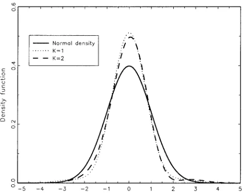
Figures 4 and 5 show the marginal densities of the distur-bances˜1 and˜2estimated under the exible parametric
den-sities and normality. Both exible parametric denden-sities have more mass close to the mode and slightly fatter tails than the normal density. The estimated standard deviation of˜1 is .64
in both theKD1 andKD2 specications, almost similar to
the estimate under normality. For the standard deviation of˜2,
we nd .89 and .90 for˜2for theKD1 and theKD2 density.
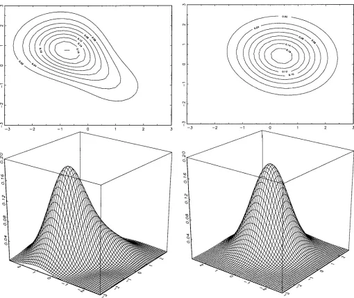
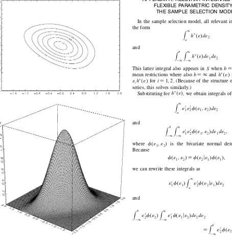
Figures 6 and 7 graph the estimated densities of the normal model and the model estimated using an exible parametric
density (KD2). We see that the estimated exible
paramet-ric density is a bit more spread out than the normal density, and that the estimated contour lines in Figure 7 are not the ellipsoids of Figure 6.
Figure 4. The Estimated Marginal Density Function of˜1.
5. CONCLUSION
In this article we have derived a test for normality in sam-ple selection models. To our knowledge, no such test has been derived previously. The test is motivated on the seminonpara-metric maximum likelihood method introduced by Gallant and Nychka (1987). A exible parametric density function is used to approximate the density function of the error terms. The bivariate normal density is a special case of this exible para-metric density function that allows us to test for normality. The test also provides an alternative density function in the event that normality is rejected.
Although the simulation study provided in this article is limited, we believe that this test is promising. The test formed well in almost all simulation experiments, the per-centage of incorrect rejections is below the signicance level, whereas the power is high. This is not true only when the
Figure 5. The Estimated Marginal Density Function of˜2.
Figure 6. Estimated Density Under the Normality Assumption.
distribution of the error terms is heteroscedastic depending on an unobserved variable. The test is powerful against departures from normality and against heteroscedasticity depending on an observed exogenous variable. However, it should be noted that in most cases the parameter estimates do not seem very sensitive to the distributional assumptions of the disturbances. Even in the event that the disturbances do not follow a normal distribution, maximum likelihood under the assumption of nor-mality provides estimates close to the true values. Only if the covariance matrix of the error terms depends on an observed exogenous variable are the parameter estimates biased. The simulation study indicates that the bias disappears when using the exible parametric density. The exible parametric density is thus useful in cases where not only parameter estimates, but also the complete distributional structure are of interest, and in the case of heteroscedasticity.
Figure 7. Estimated DensityKD2.
Finally, we have applied the normality test to a model of travel demand. The empirical results mimic those found in the simulation study; we reject the assumption of normality, but the parameter estimates turn out to be not very sensitive to the normality assumption. In this case, the exible parametric density is capable of correcting for the unobserved selectivity, which is not captured by the normal density.
ACKNOWLEDGMENTS
The authors thank Christopher Ferrall, Jean-Francois Lamarche, Jeffrey Wooldridge, an anonymous associate editor, and an anonymous referee for useful comments and sugges-tions. The Gauss code for the estimation procedure discussed
in this article can be downloaded from www.tinbergen.nl/
¹klaauw/normal.htm.
APPENDIX A: RELEVANT INTEGRALS OF THE FLEXIBLE PARAMETRIC DENSITY IN
THE SAMPLE SELECTION MODEL
In the sample selection model, all relevant integrals are of the form
Zˆ
a
hü4˜5d˜2
and
Zb
ƒˆ
Zˆ
ƒˆh ü4˜5d˜
1d˜2
This latter integral also appears inS when bD ˆ and in the
mean restrictions where alsobD ˆ andhü4˜5is replaced by
˜ihü4˜5foriD112. (Because of the structure of the Hermite
series, this solves similarly.)
Substituting forhü4˜5, we obtain integrals of the type
Zˆ
a
˜i1˜
j
2”4˜11 ˜25d˜2
and
Zb
ƒˆ
Zˆ
ƒˆ
˜i
1˜
j
2”4˜11 ˜25d˜1d˜21
where ”4˜11 ˜25 is the bivariate normal density function.
Because
”4˜11 ˜25D”4˜2—˜15”4˜151
we can rewrite these integrals as
˜i1”4˜15
Zˆ
a
˜j2”4˜2—˜15d˜2
and
Zb
ƒˆ˜
j
2”4˜25
Zˆ
ƒˆ˜
i
1”4˜1—˜25d˜1d˜2
DZb ƒˆ
˜j2”4˜25E4˜i
1—˜25d˜20
The last integral can be solved easily because
E4˜i
1—˜25Dƒ0Cƒ1˜2C¢ ¢ ¢Cƒi˜
i
20
The coefcientsƒ depend only on the other parameters of the
density function, and they are independent of˜2.
Both integrals can be calculated using the recursion formu-las that follow. Therefore, we deneIk4a1 b5as the univariate integral
Ik4a1 b5DZb
a
uk
exp4ƒu2=„25du0
Using partial integration, we obtain the recursion formulas
Ik4a1 b5D
„2
2
¡
akƒ1exp4ƒa2=„25ƒbkƒ1exp4ƒb2=„25¢
C4kƒ15„
2
2 Ikƒ24a1 b5
ifk¶2; otherwise,
whereê4¢5is the standard normal distribution function. In the
special case whereaD ƒˆandbD ˆ, the recursion formulas
simplify to
APPENDIX B: THE SIMULATION EXPERIMENTS
The simulation experiments in Section 3 were performed
as follows. For all experiments, we impose var4˜15D4,
var4˜25D1, and cov4˜11 ˜25D1.
In the rst simulation experiments, we draw˜ from either
a bivariate normal distribution with mean 0, a bivariate t
distribution, or a centered chi-squared distribution. Drawing from the bivariate normal distribution is straightforward. In the bivariate t distribution, ˜2 Du1=
p
3 and ˜1D˜2Cu2,
withu1 andu2 independent draws from at3 distribution. For
the bivariate chi-squared distribution,˜2D 1
In the last two experiments, the error terms are bivariate normal distributed but heteroscedastic. First, the distribution of
˜depends on the explanatory variablex. We dene the weight
rD1
a standard normal distribution and ˜1Dr 4˜2C
p
3u5, where
u is a realization from a standard normal distribution. For
each individual, the correlation between ˜1 and ˜2 is equal
to .5 and thus is independent of the value ofx. Furthermore, Ex6var4˜1—x57D4 and Ex6var4˜2—x57DEx6cov4˜11 ˜2—x57D1. Second, we distinguish three groups of individuals who
have different covariance matrices. The unobserved weightr
can take three values,p05, 1, and p105. The population is
over these three values. Here˜2 is again drawn from a
stan-dard normal distribution, and˜1Dr 4˜2C
p
3u5, withua real-ization of a standard normal distribution that is independent of˜2.
[Received September 2000. Revised October 2001.]
REFERENCES
Abadie, A., Angrist, J. D., and Imbens, G. W. (2002), “Instrumental Variables Estimation of Quantile Treatment Effects,”Econometrica, 70, 91–117. Ahn, H., and Powell, J. L. (1993), “Semiparametric Estimation of Censored
Selection Models With a Nonparametric Selection Mechanism,”Journal of Econometrics, 58, 3–29.
Buchinsky, M. (1998), “The Dynamics of Changes in the Female Wage Distri-bution in the U.S.A.: A Quantile Regression Approach,Journal of Applied Econometrics, 13, 1–30.
Cameron, A. C., and Johansson, P. (1997), “Count Data Regression Using Series Expansions With Applications,”Journal of Applied Econometrics, 12, 203–223.
Cosslett, S. R. (1991), “Semiparametric Estimation of a Regression Model With Sample Selectivity,” inNonparametric and Semiparametric methods in Econometrics and Statistics, eds. W. A. Barnett, J. L. Powell, and G. Tauchen, Cambridge, U.K.: Cambridge University Press.
Gabler, S., Laisney, F., and Lechner, M. (1993), “Semi-Nonparametric Maxi-mum Likelihood Estimation of Binary Choice Models With an Application to Labour Force Participation,”Journal of Business & Economic Statistics, 11, 61–80.
Gallant, A. R., and Nychka, D. W. (1987), “Semi-Nonparametric Maximum Likelihood Estimation,”Econometrica, 55, 363–390.
Heckman, J. J. (1979), “Sample Selection Bias as a Specication Error,” Econometrica, 47, 153–161.
(1990), “Varieties of Selection Bias,” American Economic Review Papers and Proceedings, 80, 313–318.
Heckman, J. J., LaLonde, R. J., and Smith, J. A. (1999), “The Economics and Econometrics of Active Labor Market Programs,” inHandbook of Labor Economics, Vol. 3, eds. O. Ashenfelter and D. Card, Amsterdam: North-Holland.
Heckman, J. J., Tobias, J. L., and Vytlacil, E. (2000), “Simple Estima-tors for Treatment Parameters in a Latent Variable Framework With an Application to Estimating the Returns to Education,” Working Paper 7950, NBER.
Hurd, M. (1979), “Estimation in Truncated Samples When There is Het-eroskedasticity,”Journal of Econometrics, 11, 247–258.
Ichimura, H., and Lee, L.-F. (1991), “Semi-Parametric Least Squares Estima-tion of Multiple Index Models: Single EquaEstima-tion EstimaEstima-tion,” in Nonpara-metric and SemiparaNonpara-metric Methods in EconoNonpara-metrics and Statistics, eds. W. A. Barnett, J. L. Powell, and G. Tauchen, Cambridge, U.K.: Cambridge University Press.
Lee, L.-F. (1978), “Unionism and Wage Rates: A Simultaneous Equations Model With Qualitative and Limited Dependent Variables,” International Economic Review, 19, 415–433.
(1982), “Some Approaches to the Correction of Selectivity Bias,” Review of Economic Studies, 49, 355–372.
Manski, C. F. (1989), “Anatomy of the Selection Problem,”Journal of Human Resources, 24, 343–360.
Melenberg, B., and van Soest, A. (1993), “Semi-Parametric Estimation of the Sample Selection Model,” working paper, CentER, Tilburg.
Newey, W. K., (1999a), “Consistency of the Two-Step Sample Selection Esti-mators Despite Misspecication of Distribution,”Economics Letters, 63, 129–132.
(1999b), “Two-Step Series Estimation of Sample Selection Models,” working paper, Massachusetts Institute of Technology.
Smith, R. J. (1989), “On the Use of Distributional Misspecication Checks in Limited Dependent Variable Models,”Economic Journal Supplement, 99, 178–192.
Tunalõ,ÇI. (2000), “Rationality of Migration,”International Economic Review, 41, 893–920.