w liv 0269 upgrade latsa software.

(1)

final re

port

p

This publication is published by Meat & Livestock Australia Limited ABN 39 081 678 364 (MLA). Care is taken to ensure the accuracy of the information contained in this publication. However MLA cannot accept responsibility for the accuracy or completeness of the information or opinions contained in the publication. You should make your own enquiries before making decisions concerning your interests. Reproduction in whole or in part of this publication is prohibited without prior written consent of MLA.

EnviroAg

Australia Meat & Livestock Australia acknowledges the matching funds provided by the Australian Government to support the research and development detailed in this publication.

In submitting this report, you agree that Meat & Livestock Australia Limited may publish the report in whole or in part as it considers appropriate.

Project code: W.LIV.0269

Prepared by: Luke Hogan & Peter Binns

EnviroAg Australia Pty Ltd

Date published: June 2010

ISBN: 9781741918304

PUBLISHED BY

Meat & Livestock Australia Limited Locked Bag 991

NORTH SYDNEY NSW 2059

(2)

Abstract

(3)

Executive summary

Version 2.0 of the Live Air Transport Safety Assessment (LATSA) software has been developed to assess the ventilation capacity of aircraft and their ability to safely dissipate generated heat, moisture and carbon dioxide. It is important to note that LATSA 2.0 models several complex systems and has been designed on a conservative basis. In many of its calculations LATSA 2.0 assumes a worse than average case scenario for constants and variables. As a result the values predicted through use of the program will in most cases, exceed what is likely to occur in practice. While this approach may over estimate temperature, humidity and carbon dioxide limits in aircraft holds in-flight, it assists exporters by clearly identifying marginal load cases. In doing so it should provide a level of confidence (including some degree of safety) on which the regulating bodies can rely.

Version 2 of LATSA is structured to meet many sometimes conflicting constraints. There is both a need for expanded storage of information and a generic simplicity in presentation and operation of the program. The program attempts to cater for both situations. The objectives of this project have expanded the table structure and computational requirements of the original LATSA software. The structure and storage requirement of both the administrative and participant areas of the database has increased at least four fold.

Version 2 of LATSA now incorporates extensive algorithms for both animal physiological factors and ventilation computations. The SQL database which forms the basis of the system is supported by source code written in ASP.NET (VB.Net). The interface is HTML based and would be familiar to almost all participants who operate in an internet based environment.

The upgrade of the program now presents the heat, moisture and carbon dioxide outputs for any single consignment of cattle, sheep and goats and any combination of these livestock. It then uses psychometric calculations together with publically available aircraft ventilation data to determine if the aircraft has the basic capability to transport the consignment without incident. Version 2 of LATSA is positioned to provide a worse than average case, meaning that if the program provides a successful result the in-flight conditions will be controllable. If the program presents a poor or bad result it is quite likely that there will be severe consequences for the animals travelling on the aircraft.

In the case of marginal or poor results from the program, it is expected that the exporter would commence discussions with the aircraft carrier to determine alternative loading conditions. While exporters are generally expert in livestock management and transportation they are not aircraft engineers and cannot be expected to have intimate knowledge of aircraft design. However, LATSA is designed to assist exporters to understand the constraints and to ask the right questions when load conditions appear unsatisfactory. For example, AQIS have concerns regarding the transport of livestock in lower holds. This concern has developed due to the dramatic variation in the ventilation capacity of lower forward and aft holds. This variation extends from very high capacity to no ventilation whatsoever. LATSA has capacity to store and utilise this and other information as it becomes available, however, administration of the database is necessary to ensure that information is accurate over time.

(4)

(5)

Success in achieving objectives ... 54

5.1 Overall success ... 54

5.2 Potential improvements in future versions ... 54

5.2.1 Monitoring data for verification of LATSA predictions ... 54

(7)

5.2.3 Boeing live animal cargo environment manuals ... 57

6

Impact on livestock industry ... 59

7

Conclusions and recommendations ... 61

7.1 Conclusions ... 61

7.2 Recommendations from project ... 61

8

Bibliography ... 63

9

Appendices... 66

9.1 Appendix 1 - List of symbols ... 66

9.2 Appendix 2 – Aircraft Data Tables used in version 2 of LATSA ... 68

9.3 Appendix 3 – Equation Flow Chart ... 72

9.4 Appendix 4 - Industry Consultation Outcomes ... 73

9.5 Appendix 5 - Completion of within scope changes ... 84

9.6 Appendix 6 – Additional Industry Comment ... 92

9.7 Appendix 7 – Response to Additional Industry Comment ... 96

9.8 Appendix 8 – LATSA V2.0 Administrators Manual ... 98

(8)

1 Introduction

This project developed from a need to upgrade and expand Version 1 the Livestock Air Transport Safety Assessment (LATSA) software. LATSA version 1 provided a preliminary assessment of the ventilation suitability of proposed consignments of livestock for transport in specific aircraft holds. The software was a simple, standalone tool designed to validate the conditions for which a specific set of livestock type could be transported by air. It was developed following a need to simplify the issues relating to Environmental Control Systems (ECS) on various models of aircraft when transporting livestock by air.

The Australian Quarantine and Inspection Service (AQIS) is the regulating body assigned to control the export of animals from Australia by any means. This duty extends to the health and well being of exported livestock. The primary welfare issues for this and the former project under which Version 1 of LATSA was developed, include:

 Stocking density; and,

 Aircraft ventilation capability and capacity.

It was determined that the outcomes of earlier projects relating to air transportation of livestock, in particular industry regulation of stock crate supply, should be incorporated into the database. This would allow a centralised storage point for most of the important data relating to air transportation of livestock. This centralisation could provide a mechanism by which the industry as a whole could improve its performance over time.

(9)

2 Project

objectives

2.1 Terms of Reference

In various industry meetings participants determined that data supporting animal and ventilation parameters within Version 1 of LATSA needed to be validated in addition to the expansion of the LATSA software to cope the multitude of load configurations. These discussions resulted in the development of the following objectives:

 Review the existing LATSA software and recommend software improvements;  Validate and amend if necessary the biological parameters used in the current model

which have been used to produce the physiological data for cattle, sheep and goats;  Extrapolate the physiological data to include all weights for cattle, sheep and goats;  Upgrade the existing software to perform the following calculations:

a. Calculate stocking densities based on ASEL [Australian Standards for the Export of Livestock] for consignments of multiple species and liveweights;

b. For the calculated stocking densities calculate total area and payload required to fit a desired consignment to ASEL standards;

c. Include a database of approved crate designs with floor area specifications for each deck (single, double, triple) and total floor area available for each crate;

d. Be able to load known classes and weights of animals to an elected type of crate, e. Be able to fill known number of crates with different species and average weights of

animals to ASEL standards.

 For all the functions listed above ensure that ventilation on aircraft can cope with the requested ASEL stocking density. Should aircraft ventilation be insufficient to cope with any of the requested ASEL stocking densities, recalculate stocking densities to ensure adequate ventilation for livestock;

 Undertake industry consultation with information providers and nominated software users to ensure software capabilities match industry expectations;

 To design the software so it can be accessed through the World Wide Web with suitable security.

(10)

3 Methodology

3.1 Project stages

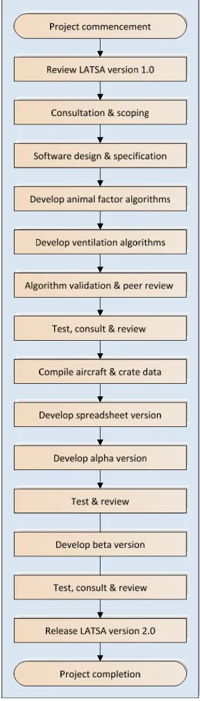
The staged approach adopted in undertaking this project is summarised in Figure 1.

(11)

3.2 Literature reviews

A literature review was undertaken to determine the most appropriate algorithms for the calculation of animal physiological parameters and the interaction with aircraft ventilation systems. The methodology adopted for this component of the project involved:

 A review of the current state of scientific knowledge in respect to the relevant physiological factors;

 Comparison of predictive relationships for physiological factors with those used in the version 1 of the LATSA software;

 Identification of suitable ‘animal factor’ algorithms for computing the required values for physiological factors applicable to all weights, ages and classes of cattle, sheep and goats;

 A review of the methodologies currently employed or potentially available for predicting the environmental conditions in aircraft ;

 Comparison of predictive relationships for environmental factors with those used in Version 1 of the LATSA software; and

 Identification of suitable ‘aircraft ventilation’ algorithms for predicting the values for key environmental variables during level flight (in cruise mode).

The key references consulted during this process include the following:  Climitization of Animal Houses (CIGR, 1992 & 2002);

 EP270.5 Design of Ventilation Systems for Poultry and Livestock Shelters (ASAE, 1986);  Live Animal Regulations (IATA, 2009a);

 Nutrient Requirements of Domesticated Ruminants (Freer et al., 2007);  Perishable Cargo Regulations (IATA, 2009b);

 SAE AIR1600: Animal environment in cargo holds (SAE Aerospace, 2003); and

 Standards for the Microclimate inside Animal Transport Road Vehicles (SCAHAW, 1999).

A more comprehensive bibliography is provided in Section 8 of this report.

It should be noted that the International Air Transport Association (IATA) regulations (IATA, 2009a & 2009b) treat SAE AIR1600 as the primary reference in these matters.

(12)

3.3 Software design and specification

A review of version 1 of LATSA established that the main areas requiring improvement were those previously identified in the terms of reference for this project (refer Section 2, above). This was reinforced by a consultative meeting held with MLA/LiveCorp staff and industry representatives in Brisbane on 16 February 2010.

In the review it was found that version 1 of LATSA consisted of hard written data tables for specific livestock types or classes together with output values. Across all species, the available livestock types were limited to less than ten selections. The number of selections was consistent with SAE AIR1600. The physiological data appear to be drawn from graph presented in literature reviewed during the originating project, and so were restricted to the few animal types represented in that material.

While version 1 of LATSA ensured that a process was in place to guide exporters (participants) through the system and provide a definitive answer, it does not have the ability to match all consigned loads. In addition the software does not provide any computational analysis of either animal physiological parameters or aircraft ventilation.

Version 1 of LATSA contained aircraft model and general capacity data but the linkages between operators and aircraft were incomplete in the basic version. The expectation was that these were to be manually updated by users or loaded via a software update. The use of lower holds, deemed important by AQIS was dealt with via a simple yes/no checkbox and the assignment of livestock to various aircraft holds was not available.

Through the review of version 1 of LATSA, and a review of the objectives, it was determined that software needed to be reconstructed, rather than simply modified. A small portion of the original Microsoft® Access database, principally the aircraft, operator and airport tables, was capable of being extracted and expanded to include all the data required to fulfil the project objectives. Version 2 of LATSA was required to be internet based. The decision was made to construct the database in an SQL environment, which required placement on an SQL server. The user interface has been written in Microsoft® Visual Studio 2, and presents itself in a similar fashion to many HTML based internet sites.

The computation analysis forming the backbone of the system is written in ASP.NET (VB Net). The intellectual property associated with the source code remains the property of Meat and Livestock Australia Limited.

The database tables have extensive inter-relationships. Many of the tables and fields are more extensive than the basic requirements of the project objectives. A decision was taken to provide some ‘future proofing’, by providing the ability to collect and store additional information, which could be utilised in future upgrades of the software. Coupled with the methodology and documentation of the source code, this will ensure that minor upgrades of the software are cost effective.

The source code encapsulates all the calculations referred to in this report. Computational results are not hard written to database table field. This allows real time correction of results when changes are made to source data (i.e. that entered by the user through the consignment window).

(13)

manipulation of important information such as hold ventilation data and crate details, much of which has a very significant impact on the results obtained in the general user area of the software. Secondly, the general user (participant or exporter) has access to the Consignment pages of the software. This allows the exporter to load all consignment information; assign crates, animals and aircraft holds through load lines; obtain results based on each hold utilised; and extract overall data such as flight time and total weight. In addition, the exporter can retrieve general consignment information and the required data for exportation documentation.

The field linkages within the table structure allow for selection of variables, such as operators, aircraft, holds, manufacturers, crates and animals in a related manner. Where data is not linked by the System Administrator, it cannot be selected. As an example, where a crate fits only one aircraft hold (e.g. Boeing 747-400 main hold) it cannot be selected in any other aircraft or hold – it will simply not be available for selection (e.g. A340-300 main hold or Boeing 747-400 lower forward hold).

In addition to field linkages, there are compliance fields within the operator, aircraft and hold tables, which restrict the use of the appropriate data if it is deemed non-compliant by industry or the regulating body. This compliance check may be as specific as one hold of one plane for one operator. Again, where data is non-compliant, it will simply not appear in the selection list.

(14)

3.4 Compilation of aircraft and crate data

3.4.1 Aircraft data

No comprehensive set of data relating to aircraft heating, ventilating and air conditioning (HVAC) systems could be located in the public domain, and some difficulties were experienced trying to source the required data from aircraft manufacturers or operators. While the report associated with version 1 of LATSA does include a quantity of HVAC data, the dataset does not include all the variables required to undertake the calculations used in version 2. Consequently, it was necessary to supplement the existing data with information that could be obtained from aircraft manufacturer’s published values (where available), values in IATA standards, and other sources. During this process the opportunity was taken to cross-check the version 1 data with other sources. If any anomalies were identified, these were investigated further and what was judged to be the best available data, whether it was the version 1 values or others, was used in version 2. A summary of the Aircraft and Hold Tables as at the time of this report can be found in Section 9.2 Appendix 2 – Aircraft Data Tables used in version 2 of LATSA.

Historically, aircraft specifications, including those pertaining to HVAC systems, have used United States customary units (US units) rather than Système International (SI) units. However, both US and SI units are now being used in these publications. As a precursor to developing the aircraft datasets used in version 2 of LATSA, all data using US units were converted to SI unit values. This included the US unit datasets in version 1 of LATSA.

3.4.2 Crate data

Much of the upgrade to LATSA is based on the issues of industry regulation of stock crates, the ability to place known numbers of crates in aircraft hold and the assignment of stock to crates to meet ASEL standards. In order to load and calculate nominated stocking densities, and compare these to ASEL, the software is required to store a significant amount of data relating to identifiable stock crates.

The data table structure includes several tables relating to the following:

 Crate Manufacturer’s detail;

 Crates details including certification information;  Tier details; and

 Hold Information.

While the information is sufficiently detailed to allow the objectives of stock assignment and stocking density calculations to be met, no manufacturer has been required to provide proprietary information that would not normally be discovered through the general use of the product. However, manufacturers and stock crates will be individually identifiable through the use of the software. This has both positive and negative consequences for all parties, but this issue is not within the terms of reference of this project.

In order to meet one objective of the project, the crate manufacturer and crate details tables include fields associated with manufacturer registration and crate certification respectively. While this information is present and is reported on output documents, it does not preclude the use of uncertified crates and unregistered manufacturers.

(15)

noted that participants may be required to develop additional knowledge of the hold assignment in order to utilise the system effectively. While this may be seen as a constraint, it is viewed as a potential requirement in meeting regulatory demands both now and in the future. A basic participant knowledge of ventilation constraints and hold structures is required in order to operate LATSA V2.0 effectively.

The number, size and configuration of crates placed in an aircraft hold are important in the calculation of volumetric data and subsequent air velocity and mixing ratios. The latter have a direct impact on the primary considerations of this project. The internal floor area of each tier and the number of stock are utilised in calculating the actual stocking density. This result is compared to the ASEL density, which the program develops from regression equations based on the ASEL standard (see Section 4.1.4).

(16)

4 Results

and

discussion

4.1 Terminology, concepts and assumptions

4.1.1 Hold nomenclature

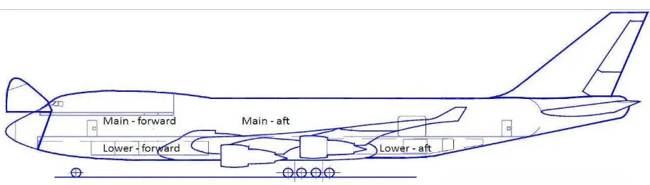
Figure 2 illustrates the names applied to aircraft holds in this report.

Figure 2: Hold nomenclature used in this report (B747-400 Freighter silhouette ©Boeing Commercial Airplane Company, 2002)

In passenger aircraft the main hold is fully utilised for passenger accommodation. In ‘combi’ configurations, the main hold is partly utilised for passenger accommodation, allowing ‘cargo only’ access to the remainder of the hold. Livestock might still be carried in the lower holds on passenger aircraft, or in the freight section of the main hold of combi aircraft, provided that adequate ventilation segregation is installed.

Not all lower holds or all parts of lower holds have the ability to carry the containerised or palletised Unit Load Devices (ULDs) normally required for livestock transport. Similarly not all lower holds on all aircraft are suitably ventilated for the transport of livestock – although this limitation generally applies more to older aircraft.

As indicated in Figure 2, in larger and multi-decked aircraft such as the Boeing B747, the main deck can consist of forward and aft zones, and ventilation may be delivered to these two zones under different regimes. However, these differences are not directly addressed in the IATA Live Animal Regulations or SAE AIR1600. While there may be some variation in air flow dynamics within the main hold this has not been taken into account in the context of the relative precision of the calculations presented in this report. In any future development and refinement of the LATSA software, consideration might be given to modelling the zonal differences in aircraft holds.

4.1.2 Livestock crates

Cattle, sheep, goats and camelids1 being exported from Australia are normally transported in single-use containers, generally made of timber, plywood and/or fibreboard. These containers can be referred to by various names (e.g. crates, pens, boxes, stalls, etc). However, to be consistent with the terminology commonly applied in the Australian livestock exporting industry, these containers are referred to, both in this document and LATSA, as crates.

(17)

To facilitate standardised handling and loading on aircraft, the external dimensions (width, length, height, profile, etc.) of livestock crates normally correspond to those of one of the standard ULDs used for air freight. Crates are designed to fit on standardised aircraft pallets (one type of ULD). These pallets are relatively thin and manufactured from aluminium to standard designs detailed in NAS 3610 – 1990. The external dimensions of most, but not all, livestock crates currently manufactured in Australia correspond to those of a PMC flat pallet ULD (also known as a P1P or LD-7). The designation of PMC can be found in Chapter 4 of the IATA ULD Technical Manual and refers to P = Pallet, M = 2,438 x 3,175mm (96 x 125 in) and C = the restraint system in our case a net system. Version 2 of LATSA includes a database of standard crates available from Australian crate manufacturers and export agents. These crates may in future also be certified as suitable for the purpose (refer MLA Project W-LIV-0261). Version 2 of LATSA has been design to store the details of all certified (and uncertified) crates.

4.1.3 Tiers

When juvenile or smaller-framed adult livestock (e.g. sheep and goats) are being transported, it is possible to use what can be described as multi-level, multi-tier, multi-floor or multi-deck crates, and still remain within the relevant loading height limitations of aircraft holds. The term tier will be used in this document when referring to these crates. Figure 3 shows an example of a 2-tier timber crate (without the entry door in place).

Tier

Side (near) Side (far)

Back Door

(removed)

Figure 3: Example of a 2-tier crate used for aircraft transport of livestock

4.1.4 Stocking density

(18)

follow the contour of the aircraft hold, further reductions in useable tier area may occur – refer ASEL standards for details of applicable reductions.

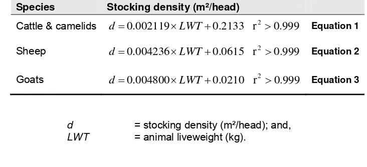
To accommodate the project requirement that version 2 of LATSA be able to calculate allowable stocking densities for all species of interest and for all likely animal liveweights, the tabulated maximum stocking densities in the ASEL standards were analysed to produce the regression equations listed in Table 1. In all three cases, the coefficient of determination (r²) values for the regression equations are effectively unity (i.e. the three equations explain all the variation in the tabulated data).

Table 1: Regression equations used to calculate maximum stocking densities for animals of various liveweights allowed under ASEL

Species Stocking density (m²/head)

Cattle & camelids

d



0

.

002119



LWT



0

.

2133

r

2



0

.

999

Equation 1

Sheep

d



0

.

004236



LWT



0

.

0615

r

2



0

.

999

Equation 2

Goats

d



0

.

004800



LWT



0

.

0210

r

2



0

.

999

Equation 3

Where: d = stocking density (m²/head); and, LWT = animal liveweight (kg).

4.1.5 Heat

Heat is a form of energy that can remain stationary in a closed, insulated system or be transferred between two bodies or connected systems and will naturally flow from a body or system at higher temperature to another at a lower temperature. This flow happens irrespective of whether the bodies are animate or inanimate. Importantly, any flow of heat energy in the reverse direction, against the natural trend, will necessitate work – in the context of physics – being done. The units applicable to a flow of heat energy are the Watt (W). A Watt is equivalent to a Joule per sec (J/s).

Heat can be considered to have two components:  Sensible heat; and

 Latent heat.

4.1.6 Sensible heat

(19)

4.1.7 Latent heat

Latent heat is ‘hidden’ heat, which is not sensed directly by humans. It is the component of total heat in a system associated with a change of state (such as occurs in evaporation, vaporisation, sublimation, condensation, etc.).

4.1.8 Total heat

Total heat is the sum of the component sensible and latent heat, and can be expressed as:

lat sen

tot







Equation 4

Where: tot = total heat;

sen = sensible heat; and

lat = latent heat.

In general, if a surface is dry, energy will be intrinsically lost (or gained) in the form of sensible heat. If a surface is wet, energy can be used to drive evaporation (provided evaporation is possible), and will therefore be lost as latent heat. If a surface is neither completely wet nor completely dry, such as the typical case for the skin of an animal, energy is normally lost as a combination of sensible and latent heat.

4.1.9 Homeothermy

Homeothermic animals attempt to maintain a constant core body temperature irrespective of the environmental conditions the animal is exposed to. This ability is involuntary. However, the efficiency of the process is neither complete nor uniform across all species, ages, classes and conditions of homeothermic animals.

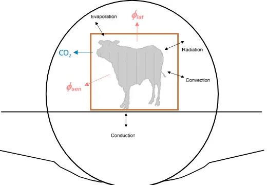
Figure 4 illustrates the thermal interactions between an animal and the environment within an aircraft hold. These interactions represent those involved in the animal attempting to maintain a constant core body temperature (i.e. homeothermy). The normal mechanisms for heat transfer in such circumstances are radiation, convection and conduction (i.e. sensible heat), and evaporation2 (i.e. latent heat).

(20)

Figure 4: Diagrammatic representation of the interaction between a transported animal and the environment in an aircraft hold

Importantly, the flow of energy is not uni-directional, and depending on environmental conditions may involve the animal not simply dissipating, but also assimilating some energy. For example, heat will be gained by radiation or conduction, rather than lost, if an animal’s surroundings (e.g. the aircraft hull) are hotter than the outside surface (skin) of the animal.

4.1.10 Effects of temperature & humidity on heat transfer

By way of example the observed effects of ambient air temperature and relative humidity on total, sensible and latent heat transfers in an experiment involving Ayrshire bull claves are depicted in Figure 5 (ASAE, 1986).

10 20 30 40

Air temperature (°C) -100

0 100 200 300

Hea

t lo

s

(

J

/s

)

Total losses

Latent heat losses

Sensible heat losses

0 20 40 60 80 100

Relative humdity (%) -100

0 100 200 300

Total losses

Latent heat losses

Sensible heat losses

(21)

While the magnitude of the total sensible and latent heat losses reported here are specific to the Ayrshire calves used in the subject experiment, due to the degree of commonality in the physiological regulation mechanisms involved, not entirely dissimilar trends are likely to be seen in other ages and species of mammalian (homeotherm) livestock.

The following are noteworthy in respect to Figure 5:

 Total heat losses were relatively uniform – although not entirely so – under the temperature and humidity conditions experienced in the subject experiments;  When conditions aside from ambient temperature were held constant, sensible heat

losses decreased and latent heat losses increased with increases in temperature;

 When the temperature was 35°C, and conditions other than humidity were held constant, sensible heat losses increased and latent heat losses decreased with increases in relative humidity;

 The experiments did not explore the potentially contrary effects on sensible and latent heat losses that may result from concurrent increases or decreases in temperature and relative humidity;

 The experiments did not evaluate the effects of air speed in the animal’s environment; and

 Potential complicating factors such as activity levels, degree of acclimatisation, body condition, dietary energy intake, growth rates etc., were not explicitly considered.

4.1.11 Thermoneutrality

Homeothermic animals, such as domestic ruminants, need to maintain their core body temperature within the range of 38 to 39°C to allow vital physiological processes to take place. This core body temperature is maintained by a combination of metabolic activity and certain physiological and behavioural responses (Freer et al., 2007 and Hillman, 2009).

The range of environmental conditions over which an animal can maintain its core body temperature with minimal thermoregulatory effort (i.e. thermoneutral conditions) is finite. Thermoneutral conditions are commonly depicted as a distinct ‘thermoneutral zone’, bound at its upper and lower limits by what are generally termed the upper and lower critical temperatures, or UCT and LCT (refer CIGR 1992; CIGR 2002; Freer 2007 and Hillman, 2009). Outside of these temperature limits, the animal notionally begins to be exposed to heat and cold stress respectively3.

Heat production is likely to increase due to exposure to both heat and cold stress – which can be somewhat counterproductive in the case of heat stress. Ongoing exposure to heat or cold stress will result in hyperthermia or hypothermia respectively, and without any respite, may ultimately result in death. Where there is regular or ongoing exposure to moderately stressful conditions, animals do have the capacity to acclimatise or adapt to those conditions (e.g. animals from tropical areas might have a higher UCT than those from more temperate areas).

3_{An alternative concept to that of a thermoneutral zone bound by a UCT and a LCT is one of a}

biologically

optimum temperate, where an animal is, on average, under the least amount of thermal stress (refer

(22)

Figure 6 provides a classical representation of the conceptual relationship between heat production, a thermoneutral zone and upper and lower critical temperatures. In practice this relationship is more complex than Figure 6 suggests – particularly in regard to heat stress. However, within the context of this review, the relationship depicted is reasonably sound.

Environmental temperature R at e o f h e a t p rod u ct ion o r l os s Summit metabolism Lower critical temperature Upper critical temperature Thermoneutral zone

Evaporative heat loss

Sensible heat loss Heat production Cold thermogenesis Hyp o th e rmi a H y pe rthe rmia

Figure 6: Notional effects of environmental temperature on thermoregulation in livestock (adapted from Freer et al., 2007)

Within the thermoneutral zone in Figure 6, the relationship between the total, sensible and latent heat produced by an animal is analogous to that depicted in the left-hand graph in Figure 5 (page 20), with sensible heat losses decreasing and latent heat losses increasing as the ambient temperature progressively increases.

A major objective in managing the environment in an aircraft hold used to transport livestock must then be to minimise the risk of the animals being exposed to unnecessary thermal stress. Hence, that environment should ideally be kept within the thermoneutral zone of the transported animals. However, neither upper nor lower critical temperatures can be represented by a fixed value – this is indicated by the lack of a defined numerical scale on the x-axis in Figure 6. The relevant values for both temperatures vary with a diverse range of factors including:

 Species and genotype;  Age;

 Liveweight;  Growth rate;

(23)

 Depth of coat or fleece;  Skin wetness and humidity;  Air speed (environmental); and  Acclimatisation.

4.1.12 Critical temperatures

Despite its depiction as a well-defined, discrete point in Figure 6 (above), there is no unequivocal physiological definition of the temperature representing the upper critical temperature (UCT). However, one widely accepted definition is that of the IUPS Thermal Commission (2001), which is:

‘The ambient temperature above which the rate of evaporative heat loss in a resting thermo-regulating animal must be increased (e.g. by thermal tachypnoea4 or by thermal sweating), to maintain a thermal balance’

Other definitions of UCT typically relate to it being the temperature at which an increase is observed in metabolic heat production as a result of the muscular expenditure involved in panting (i.e. the upwards inflection point in the red plotline on the right-hand side of Figure 6). However, while an observable increase in metabolic heat production as panting commences is common, it is not necessarily a universal characteristic of endothermic animals5 (see Hillman, 2009).

As ambient temperatures drop below the lower critical temperature (LCT), there is a compensatory increase in the rate of metabolic heat production, principally as a result of shivering and/or non shivering thermogenesis. Any increase in metabolic activity has physiological limits, and can neither be sustained indefinitely nor always be sufficient to compensate entirely for the cold conditions. Behavioural changes such as huddling or adopting curled lying positions, which minimise the exposed surface area from which radiative transfers can occur, may be adopted in an attempt to reduce heat losses, provided that any physical constraints (e.g. stocking density) permit such activity. In an increasingly cold environment, shivering and non-shivering thermogenesis will, in time, fail to have a sufficient compensatory effect, and core body temperature will begin to drop. Eventually hypothermia will set in. Again, in the absence of any timely respite, death will ultimately occur.

4.1.13 Respiratory quotient

Metabolic activity results in an animal consuming atmospheric oxygen (O2) and respiring carbon dioxide (CO2). The respiratory quotient (RQ) is the ratio of the volume of CO2 eliminated, to the volume of O2 consumed, and varies with the organic substrates (carbohydrates, proteins, fats, etc.) being metabolised. The following stoichiometric equations are recognised mechanisms for the metabolism of glucose (C6H12O6) and a fat (C51H98O6), and depict how the proportions of O2 consumed and CO2 generated vary with the substrate being metabolised6.

4_{Unusually fast breathing (}

i.e. panting) to enhance latent heat loss from the respiratory tract

5_{Mammalian and avian animals, including livestock, that maintain their relatively high body temperatures} by metabolic heat production

6

(24)

MJ 32 O 49H 51CO 71.5O O H C MJ 2.82 O 6H 6CO 6O O H C 2 2 2 6 98 51 2 2 2 6 12 6        

The respiratory quotient (RQ) is 1.0 for glucose (6 moles O2:6 moles CO2), and around 0.7 for fats (0.71 for C51H98O6 in the above example). The RQ values for the more chemically diverse proteins are typically in the range of 0.8 to 0.9.

Owing to the proportions of carbohydrate, fat and protein in a balanced diet having a reasonable level of consistency, it is possible to relate CO2 production to total energy comsumption with an acceptable level of reliability – particularly where an animal is not subject to any nutritional stress and its basic nutritional requirements are being fully met (Pedersen et al., 2008).

4.1.14 Units

(25)

4.2 Animal factor algorithms

4.2.1 Lower critical temperature

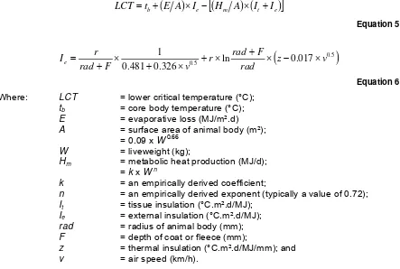
Freer et al. (2007) provide two interrelated equations for predicting lower critical temperature (LCT) in ruminants. These were used in version 2 of LATSA and are given by the following:





e





m

 

t e





b

E

A

I

H

A

I

t

LCT













Equation 5



0.5



5 .

0 ln 0.017

326 . 0 481 . 0 1 v z rad F rad r v F rad r

I_e      

     Equation 6

Where: LCT = lower critical temperature (°C); tb = core body temperature (°C); E = evaporative loss (MJ/m².d) A = surface area of animal body (m²);

= 0.09 x W0.66

W = liveweight (kg);

Hm = metabolic heat production (MJ/d); = k x W n

k = an empirically derived coefficient;

n = an empirically derived exponent (typically a value of 0.72); It = tissue insulation (°C.m².d/MJ);

Ie = external insulation (°C.m².d/MJ); rad = radius of animal body (mm); F = depth of coat or fleece (mm);

z = thermal insulation (°C.m².d/MJ/mm); and v = air speed (km/h).

The above equations assume – not unreasonably – that even under calm conditions some air movement occurs, and therefore a minimum airspeed of 0.36 km/h (0.1 m/s) applies. Applying airspeeds lower than this limit may result in erroneous estimates from Equation 6.

Of those listed above, acclimatisation is the principal factor not incorporated into the above equations.

(26)

Table 2: Comparison of lower critical temperatures (°C) under calm dry conditions predicted using Equation 5 and Equation 6 (Freer et al, 2007), with values given in NRC (1981) and SCAHAW (1999)

Species Class or condition Freer et al NRC SCAHAW

Cattle* newborn calf 14 9 10

1 month old calf 2 0 0

beef cow -12 -21 5 to -40

dairy cow, high milk yield -37 -40 -24 to -30

Sheep newborn lamb 22 — 10

shorn ewe, 5 mm wool 18 18 15

ewe, 50 mm wool -7 9 -9 to -15

*European cattle or Bos primigenius taurus

Some of the minor disparity evident between the same species in Table 2 appears due to a lack of consistency between the sources in respect to the energy intake (e.g. fasting vs. maintenance vs. ab libitum feed supply), coat or fleece depth, growth rate, milk yield, age, weight, etc. within the same class of animal. In some cases, the applicable values for these parameters are not stated in the different sources, and consequently any standardisation is difficult.

4.2.2 Upper critical temperatures

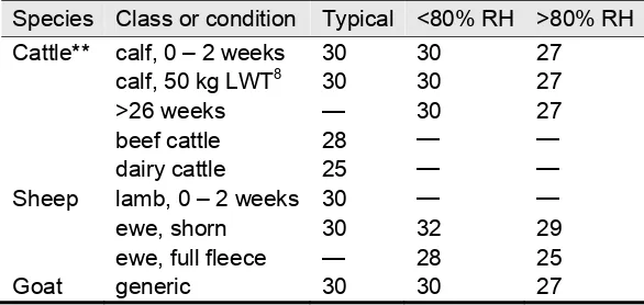
Unfortunately upper critical temperatures do not lend themselves as easily as lower critical temperatures to their estimation using simple predictive equations. However, tabulated values are published in scientific literature. The tabulated UCT values used in version 2 of LATSA, and which have been taken from Standards for the Microclimate inside Animal Transport Road Vehicles (SCAHAW, 1999), are listed in Table 37.

Table 3: Upper critical temperatures (°C) for cattle, sheep and goats (SCAHAW, 1999)

Species Class or condition Typical <80% RH >80% RH Cattle** calf, 0 – 2 weeks 30 30 27

calf, 50 kg LWT8 30 30 27

>26 weeks — 30 27

beef cattle 28 — —

dairy cattle 25 — —

Sheep lamb, 0 – 2 weeks 30 — —

ewe, shorn 30 32 29

ewe, full fleece — 28 25

Goat generic 30 30 27

**European cattle or Bos primigenius taurus

(27)

4.2.3 Total heat production

Possibly reflecting a more widespread need to house grazing animals indoors during winter, much of the scientific literature pertaining directly to heat production in livestock (other than pigs or poultry) originates from North America and Europe. The Design of Ventilation Systems for Poultry and Livestock Shelters (ASAE, 1986) and Climitization of Animal Houses series (CIGR, 1992 & 2002) appear to be the more commonly cited documents in this regard.

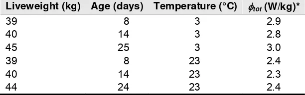
ASAE (1986) provide tabulated values for total (and sensible) heat, compiled from a number of individual studies involving various classes, ages and liveweights of livestock species, housed at various ambient temperatures9. An example relating to male Ayrshire calves, and taken from Table 1 in ASAE (1986), is reproduced here in Table 4.

Table 4: Total heat production in male Ayrshire calves (source ASAE, 1986)

Liveweight (kg) Age (days) Temperature (°C) tot (W/kg)*

39 8 3 2.9

40 14 3 2.8

45 25 3 3.0

39 8 23 2.4

40 14 23 2.3

44 24 23 2.4

* W/kg = Watts per kg LWT. 1 Watt = 1 Joule/second (J/s)

As can be seen from Table 4, the general application of the tabulated ASAE (1986) data requires some degree of interpolation and extrapolation. Discrete tabulated values do not lend themselves to direct usage in the LATSA software, although it is possible to fit regression equations to the tabulated values to facilitate interpolation and extrapolation. However, the fitting of species-specific regression equations is constrained by it being unclear as to what extent the reported differences between the values for different genotypes in the ASAE data are due to the normal stochastic variability about mean values for that species, as opposed to statistically significant or ‘true’ differences between genotypes.

In contrast to the approach in ASAE (1986), the more recent CIGR (2002) publication provides a series of predictive equations for total heat. These equations relate to a relatively comprehensive range of livestock species, and are based on the likely basal metabolisable energy requirements of the animals10. The metabolisable energy requirements are modified by additional terms in the equations to account for factors such as current growth rate, milk production and stage of foetal development (if applicable). To some extent, the accounting for differences in growth rate or milk production may coincidentally account for some genotype differences – perhaps overcoming one of the issues with the tabulated ASAE (1986) data. Table

9_{As the data are compiled from numerous studies, these temperatures are not consistent between species} or classes of species. Some of the listed temperatures are also likely to be outside of the thermoneutral range for the animals involved.

(28)

5 lists the equations for total heat production provided in CIGR (2002) for species of interest in this review.

Table 5: Predictive equations for total heat production in livestock (CIGR, 2002)

Species Class or condition

tot (W)

Cattle Calf





2 2 70 . 0 3 . 0 1 0188 . 0 28 . 6 3 . 13 44 . 6 y LWT y LWT

tot _ _

      



Equation 7

Lactating/pregnant cow 3 5 1 75 . 0 10 6 . 1 22 6 .

5 LWT y p

tot       





_{Equation 8}

Sheep Lamb 2 75 . 0 145 4 .

6 LWT y

tot    



_{Equation 9}

Lactating/pregnant ewe 3 5 1 75 . 0 10 4 . 2 33 4 .

6 LWT y p

tot       





_{Equation 10}

Goat Generic ₆_.₃ _LWT0.75 tot  



_{Equation 11}

Lactating goat

1 75 . 0 ₁₃ 5 .

5 LWT y

tot    



_{Equation 12}

Where: LWT = individual animal liveweight (kg); y1 = milk production (kg/day);

y2 = daily liveweight gain (kg/day); and p = stage of gestation (days post-mating).

Notionally, the above predictive equations for total heat production only pertain to thermoneutral conditions. CIGR (2002) provide considerable discussion as to whether certain generic and species-specific linear or curvilinear relationships provide the best fit when adjusting predictions for ambient temperatures that are outside of the thermoneutral range. Assuming that the aim of managing the environment in the aircraft hold is to maintain temperatures within the thermoneutral range, these relationships for temperatures outside the thermoneutral range are not discussed here.

Compared to other approaches, the potential advantages of the CIGR (2002) equations listed in Table 5 are as follows:

 Their more recent development suggests that they should be based on a more extensive body of scientific literature;

 Being equations, they obviate the specific computational need to interpolate between or extrapolate from the discrete tabulated values in ASAE (1986); and

 The incorporation of terms for variables other than body weight into equations should allow easier incorporation of these factors into estimates of total heat production.

(29)

4.2.4 Sensible heat loss

ASAE (1986) provide tabulated values for sensible heat loss corresponding to the tabulated total heat values discussed above.

GIGR (2002) provide the following generic relationship for estimating sensible heat loss from total heat production:

2 38 . 0 8 .

0 tot t

sen  



 



Equation 13

Where: sen = sensible heat loss (W/hpu);

tot = total heat production (W/hpu); and t = ambient temperature (°C).

The unit W/hpu represents Watts/heat production unit. A ‘heat production unit’ is a standardised unit adopted by the Commission Internationale du Génie Rural (CIGR), and which represents a group of animals – of whatever makeup – that produces 1 000 W of total heat (tot) at 20°C. To undertake the calculations on an individual animal basis (i.e. W/animal), it is necessary to revert to the comparable formula for sensible heat given in CIGR (1992), which is:







7 4



10

85

.

1

8

.

0













t

tot sen



Equation 14

Where: sen = sensible heat loss (W/animal);

tot = total heat production (W/animal); and t = ambient temperature (°C).

Although not explicitly stated, the above relationships presumably represent curvilinear regression equations that have been fitted to data similar that in the left-hand graph in Figure 5 (page 20).

It might also be noted that near the midpoint in the thermoneutral range (i.e. ~20°C in most cases), sensible heat would effectively represent around two thirds of total heat output. Conversely, latent heat would represent about one third of total heat output at such temperatures.

Similar benefits and disadvantages in respect to the use of tabulated values and equations for total heat production apply to the above methods of estimating sensible heat loss.

4.2.5 Moisture loss in the form of water vapour

(30)

CIGR (2002) provide no specific means of estimating either latent heat or moisture loss. However, if values for both total and sensible heat are known, latent heat loss (lat) can then be estimated from Equation 4 on the basis that:

sen tot

lat







Equation 15

From first principles it then follows that moisture loss can be estimated from predicted latent heat loss, and the known latent heat (i.e. vaporisation enthalpy) of water. In version 2 of LATSA this estimation is achieved using the following equation:

3600  







lat

animal

Equation 16

Where: animal = moisture loss (g/hr/animal);

lat = latent heat loss (W/animal); and

 = latent heat of vaporisation at temperature t°C (kJ/kg)

= 2501 – 2.36 x t (kJ/kg)

It should be noted here that all reference to moisture loss by respiration is in the form of water vapour. That vapour will only condense to liquid if the pyschrometric conditions are favourable.

4.2.6 Carbon dioxide production

This relationship between CO2 production and total heat can then be expressed by the following equation (CIGR, 2002):

tot pr k

C  



Equation 17

Where: Cpr = CO2 production;

k = a respiratory quotient dependent coefficient; and

tot = total heat production.

Various units can be applied to the above equation; although comparable units must be applied to the individual variables in any one computation.

CIGR (2002) indicated that for RQ values of 0.8 to 1.2, values for k of between 0.142 to 0.195 m³/hr/hpu 11 had typically been used up to that time, with a generic value of 0.163 m³/hr/hpu being commonly applied. However, evidence was by then accumulating which suggested these values represented modest underestimates. Pedersen et al. (2008) subsequently suggested that 0.185 m³/hr/hpu was a more suitable generic value for k, with the values in the range of 0.160 to 0.210 m³/hr/hpu being applicable where RQ values were known and in the range of 0.9 to 1.2.

(31)

4.2.7 Animal activity and behaviour effects

The preceding heat production or loss equations assume that the animal is in a resting state. Energy expenditure associated with increased animal activity is, however, going to affect the total heat produced. A need to compensate for aircraft movement12 or behavioural responses to any stress associated with handling and transport can cause increased levels of physical or metabolic activity – albeit often only of a transient nature – with a commensurate increase in total heat production.

SAE AIR1600 (SAE Aerospace, 2003) recommends that the total heat production of animals during loading and handling may increase up to 4 to 5 times that produced during rest. In version 2 of LATSA the potential for an increase in total heat production due to the above has been accommodated by the incorporation of an ‘behaviour factor’, which is applied to estimates of total heat production (and thus in turn affects sensible and latent heat loss values). Given industry comment in regard to on-board animal handling practices and in-flight temperature feedback, a value of 10% has been used (i.e. actual tot = 1.1 x resting tot).

4.2.8 Manure and bedding moisture

Evaporation from voided animal faeces and urine – collectively termed ‘manure’ here – can make a significant contribution to atmospheric moisture levels in a confined environment (SCAHAW, 1999).

The evaporative flux rate will depend in part on the manure temperature and moisture content, as well as the ambient temperature, air speed and humidity or vapour pressure (Liberati & Zappavigna, 2005). The exposed surface area (evaporative interface) of the manure will also influence areal evaporation rates (i.e. when expressed as g H2O/m²/hr or similar). As part of a large, integrated, animal housing model, Liberati & Zappavigna (2005) provide the following relationship for estimating evaporative losses from manure:

pw

R

a

S

_d

manure





0







Equation 18

Where: manure = evaporation from manure (kg/s); Sd = manure surface area (m²);

a0 = evaporation coefficient (7.12 – 26.6 kg/m²/hr/Pa); R = ventilation rate (m³/s); and

pw = vapour pressure differential (Pa) between the air and evaporative surface.

Equation 18 is used in version 2 of LATSA. Sd is equivalent to the total floor area of all tiers in a consignment. In practice, crates do not become fully saturated until sometime during a flight. In addition, no attenuation systems have been considered in the software although access to an reductionattenuation constant could be provided. As a result, the approach adopted in version 2 of LATSA may generate a higher value for manure than occurs in practice, which in turn may result in a higher relative humidity result than in practice.

(32)

4.3 Aircraft ventilation algorithms

4.3.1 Energy and mass balance

SAE AIR1600 (SAE Aerospace, 2003) recommends energy and mass balance approaches to estimating environmental variables in aircraft holds carrying livestock. Such approaches are based on the ‘laws’ of the conservation of mass and energy. These laws can be expressed as a standard mass or energy balance equation having the form:

Equation 19

While SAE AIR1600 provides equations for calculating humidity and CO2 levels in ventilated holds, it recommends heat balance calculations for estimating hold temperatures. One limitation of this approach is the difficulty of quantifying variables, such as heat loss or gain through the aircraft skin, using the scant information available in the public domain.

Under cruise conditions, SAE AIR1600 treats ventilation air in pressurised aircraft as the dominant sink for sensible and latent heat, and aside from leakage, the sole means of removing CO2. SAE AIR1600 also assumes that conditions will approach a steady state under cruise conditions. Thus, it is not unreasonable to consider an aircraft analogous to any other form of livestock housing, and the approaches to energy and mass balance modelling used in designing such housing should be capable of being applied to the prediction of environmental conditions in aircraft holds accommodating livestock.

The ASAE Standard EP270.5 Design of Ventilation Systems for Poultry and Livestock Shelters (ASAE, 1986) provides generic energy and mass balance equations for use in estimating ventilation requirements in livestock housing. Expressed in terms of the associated change in air temperature and mixing ratio, these equations are shown below as Equation 20 and Equation 21 respectively. v p sen n F c T T  

 ₀



Equation 20

Where: Tn = outflow temperature (°K or °C); T0 = inflow temperature (°K or °C);

sen = sensible heat exchanged13 in ventilation air (W or J/s); cp = specific heat of moist air (J/kg/°K); and

Fv = ventilation rate (kg/s).

v total n

F r

r  ₀ 



Equation 21

Where: rn = outflow mixing ratio (water:air as g/kg); r0 = inflow mixing ratio (water:air as g/kg);

total = total water vapour generated by the load through respiration (cargo) and evaporation (manure) (g/s); and Fv = ventilation rate (kg/s).

(33)

The approach adopted in Equation 21 can similarly be applied to the mass balance of CO2 within each hold.

While Equation 20 and Equation 21 are not used directly in LATSA V2.0 they provide the basis of the mass balance approach which is utilised in Sections 4.3.2 to 4.3.4 and further in Section 4.4 to generate environmental system equations which LATSA V2.0 uses to provide specific results for temperature, relative humidity and CO2 concentration.

4.3.2 Sensible heat loading

Assuming steady state conditions and parameterising the energy balance form of Equation 19, the sensible heat14 balance within an aircraft hold can then be expressed as:

v s s s s

s



 _cargo _skin ₀

Equation 22

Where: s v = sensible heat in ventilation system outflow (W);

s 0 = sensible heat in ventilation system inflow (W);

scargo = sensible heat generated by cargo (W); and

s skin = sensible heat gain (+) or loss (-) through the aircraft skin (W).

Rearranging Equation 20 (page 32), the sensible heat exchange associated with a temperature change can be expressed as:

) (T T₀ F

c_p _v _n

s    



Equation 23

If it is assumed that the amount of sensible heat transferred through the aircraft skin is not significant then when expressed in terms of more appropriate or readily quantified variables, Equation 22 becomes:



1









cargo







0



1







h _p _s _v _p _n

n

c

F

c

T

V

T







Equation 24

Where: Tn = hold air temperature (°K) at time n;

Tn-1 = hold air temperature (°K) at time n-1; Vh = hold headspace volume (m³);

ρ = density of hold headspace air (kg/m³); cp = specific heat of moist air (J/kg.°K);  = nominal time increment (s); and T0 = influent air temperature (°K).

To ignore skin losses is a relatively conservative assumption, since we are considering the maximum allowable sensible heat load under cruise conditions15 when it is more likely sensible heat will be lost rather than gained through the aircraft skin.

14

(34)

Rearranging the terms in the above equation, the hold temperature at time n can be determined as:









p h n p v s n n

c

V

T

c

F

T

c o

























₀ ₁

1

arg

Equation 25

Equation 25 is analogous to those commonly used in similar transient animal environment models – e.g. Panagakis & Axaopoulos (2004), Aerts & Berckmans (2004) and Sun & Hoff (2009).

As the sensible heat load generated by the cargo (scargo) at any one time is not constant, but dependent upon the antecedent hold temperature (Tn-1), both Tn and scargo need to be calculated on an iterative basis. However, as the estimates here pertain to cruise conditions, where the hold environment should generally approach a steady state, for computational simplicity it is possible to curtail the calculations once Tn and Tn-1 converge to within some nominal limit (e.g. the difference is less than say 0.01%). Owing to its interdependence on temperature, the value of scargo in Equation 25 will likewise have stabilised at the point of convergence. If the variable



then represents the length of the cruise phase of the flight (in units of ), the resulting iterative computational algorithm can be stated as:













n n n n p h n p v s n n T n T T T c V T T c F T T n o c Read Next else End, then , 0001 . 0 If 1 For 1 1 0 1 arg                 









Equation 26

Equation 26 is used in version 2.0 of LATSA to calculate the exit air temperature of the hold. It should be noted that this stable exit temperature is not the average temperature of the air in the hold and that the average temperature experienced within the hold may be somewhat lower due to the positioning and direction of cold inlet airflows. Modelling of airflow within the hold and around cargo was not part of the project scope.

15

(35)

4.3.3 Latent heat and moisture load

Following a mass balance approach in lieu of the energy balance one used above to estimate the steady state hold temperature (refer Section 4.3.2), the steady state mixing ratio for water in the air in the aircraft hold can be predicted using the following iterative relationship:













n n n n h n v o c n n r n r r r V r r F r r n Read Next else End, then , 0001 . 0 If 1 For 1 1 0 arg 1               









Equation 27

Where: rn = mixing ratio (g/kg) at time n; rn-1 = mixing ratio (g/kg) at time n-1;

cargo = water vapour load (g) emitted by cargo; and r0 = mixing ratio (g/kg) of influent air.

Although Equation 27 is directly utilised in version 2.0 of LATSA, it remains an intermediary step to generating a more easily understood result for Relative Humidity (see Section 4.4.3)

4.3.4 Carbon dioxide concentration

As with sensible heat and water vapour, the carbon dioxide (CO2) balance in the hold can be predicted using the following relationship:













n n n n h n v o c n n C n C C C V C C F CO C C n Read Next else End, then , 0001 . 0 If 1 For 1 1 0 arg 2 1              



Equation 28

Where: Cn = CO2 concentration (mg/m³) at time n; Cn-1 = CO2 concentration (mg/m³) at time n-1; CO2 cargo = CO2 emitted by cargo (mg/s); and

C0 = CO2 concentration (mg/m³) in influent air.

(36)

4.4 Secondary psychrometric calculations for aircraft ventilation

4.4.1 Consignment “flags”

A group of parameters discussed in this section were considered as “flags” for allowable

consignment conditions. These parameters included Effective Temperature (ET), Upper Critical Temperature (UCT) and Wet Bulb Temperature (WBT). The results of the various calculations for these parameters are included in the ESC results for each hold. However, the validity of using various parameters as black and white decision factors for what is considered short haul transportation is questionable. In particular, high ET values for flights of eight to ten hours do not present a significant issue unless those conditions were present before the flight and continue for a considerable time after the flight (i.e. days not hours). Of all the parameters, WBT was chosen as the primary (go / no-go) decision factor in Version 2 of LATSA primarily because of its

acceptance in the HotStuff software used in assessment of sea freight of livestock shipments. While parameters such as Temperature Humidity Index (THI) and UCT remain in the ECS results they are provided as guidance only and should not be considered as primary decision factors regarding consignments.

Many of the preceding computations rely on known or calculated values for various psychrometric or environmental variables. The standard equations used to calculate the specific heat of air, mixing ratio, and air density are detailed below as well as the most appropriate methodologies for other parameters found in the literature review process (see Section 3.2).

4.4.2 Specific heat of air

The specific heat of moist air (cp) is given by:



r



c

_p



_pd



1



1

.

84



10

3



Equation 29

Where: cpd = specific heat of dry air (J/kg/°K);

= 1004.67 J/kg/°K; and

r = mixing ratio of water vapour (g/kg).

4.4.3 Mixing (humidity) ratio

The mixing ratio of water vapour in the hold atmosphere can be determined (with reasonable accuracy) on the basis:

100 or 100 s s r RH r r r RH     Equation 30

Where: RH = relative humidity (%); and rs = mixing ratio at saturation (g/kg).

(37)

Equation 31

Where: es = saturation vapour pressure (kPa).

            _      T K K

e_s 1

273 1 5423 exp 611 . 0 Equation 32

Where: T = temperature (°K).

4.4.4 Air density

In level flight, the atmospheric pressure in the cabin and pressurised holds of a modern aircraft are less than at sea level. The density of air in an aircraft hold under cruise conditions can therefore be determined as:

sl sl P P



  Equation 33

Where: ρ = density of air in the aircraft hold (kg/m³); P = atmospheric pressure in the aircraft hold (kPa); Psl = atmospheric pressure at sea level (kPa); and

ρsl = density of air at sea level (kg/m³).

The density of air at sea level is normally assumed to be 1.225 kg/m³, and the atmosp