Full Terms & Conditions of access and use can be found at
http://www.tandfonline.com/action/journalInformation?journalCode=ubes20
Download by: [Universitas Maritim Raja Ali Haji] Date: 11 January 2016, At: 19:15
Journal of Business & Economic Statistics
ISSN: 0735-0015 (Print) 1537-2707 (Online) Journal homepage: http://www.tandfonline.com/loi/ubes20
Booms, Busts, and Normal Times in the Housing
Market
Luca Agnello, Vitor Castro & Ricardo M. Sousa
To cite this article: Luca Agnello, Vitor Castro & Ricardo M. Sousa (2015) Booms, Busts, and Normal Times in the Housing Market, Journal of Business & Economic Statistics, 33:1, 25-45, DOI: 10.1080/07350015.2014.918545
To link to this article: http://dx.doi.org/10.1080/07350015.2014.918545
Accepted author version posted online: 07 May 2014.
Submit your article to this journal
Article views: 406
View related articles
Booms, Busts, and Normal Times in the Housing
Market
Luca A
GNELLODepartment of Economics, Business and Statistics (SEAS), University of Palermo, 90128 Palermo, Italy
Vitor C
ASTROFaculty of Economics, University of Coimbra, Coimbra 3004-512, Portugal;
Economic Policies Research Unit (NIPE), University of Minho, Campus of Gualtar, Braga 4710-057, Portugal
Ricardo M. S
OUSADepartment of Economics and Economic Policies Research Unit (NIPE), University of Minho, Campus of Gualtar, Braga 4710-057, Portugal; LSE Alumni Association, London School of Economics and Political Science, London WC2 2AE, United Kingdom ([email protected], [email protected])
We assess the existence of duration dependence in the likelihood of an end in housing booms, busts, and normal times. Using data for 20 industrial countries and a continuous-time Weibull duration model, we find evidence of positive duration dependence suggesting that housing market cycles have become longer over the last decades. Then, we extend the baseline Weibull model and allow for the presence of a change-point in the duration dependence parameter. We show that positive duration dependence is present in booms and busts that last less than 26 quarters, but that does not seem to be the case for longer phases of the housing market cycle. For normal times, no evidence of change-points is found. Finally, the empirical findings uncover positive duration dependence in housing market booms of European and non-European countries and housing busts of European countries. In addition, they reveal that while housing booms have similar length in European and non-European countries, housing busts are typically shorter in European countries.
KEY WORDS: Change-points; Duration analysis; Duration dependence; Housing booms and busts; Weibull model.
1. INTRODUCTION
Following the burst of the technology bubble in the early 2000s, housing prices followed an unsustainable growth path in a large number of countries. However, as the subprime mortgage market crisis emerged in the summer of 2007 and the world economy witnessed the Great Recession, prices collapsed giving rise to a long and persistent slump in the housing market.
Against this background, investigating the behavior of the housing sector, the determinants of the boom–bust phases were brought into the forefront of the policymaking agenda (Agnello and Schuknecht2011). Similarly, understanding the characteris-tics of the housing cycles and their likely impact on the macroe-conomy and the financial system has gained a renewed interest from academics and researchers (Afonso and Sousa2011,2012). The recent research on the topic has shown that the likeli-hood of an ending in a given housing market cycle depends on its age, that is, as time goes by, the probability that a housing boom (upturn) comes to an end increases. As for housing busts (downturns), no evidence of such positive duration dependence has been found (Cunningham and Kolet2011). Bracke (2013) used a discrete-time duration model and also suggested the ex-istence of lagged duration dependence, as housing downturns are less likely to end when the previous upturn was abnormally long.
Our article is highly indebted to and simultaneously inspired by the aforementioned works. In particular, we aim at answering relevant questions such as: How long are housing booms, busts, and normal times likely to last? How similar (or different) are these phases between European and non-European countries? Does the end of a housing boom or bust depend on its own age? Is the duration of housing market cycles smooth or bumpy, that is, is there evidence supporting the presence of a change-point in the duration dependence of booms or busts in the housing prices? How has the duration of housing market cycles evolved over time? Therefore, we try to make one step forward in that we assess the extent to which the likelihood of a boom, bust, or normal time coming to an end changes after a certain duration. More specifically, not only do we consider that the likelihood of a housing market phase ending increases over time, but we also allow it to change when it has already lasted for more than a certain duration. To the best of our knowledge, our article pro-vides the first assessment of this second dimension of housing
© 2015American Statistical Association
Journal of Business & Economic Statistics
January 2015, Vol. 33, No. 1 DOI:10.1080/07350015.2014.918545
Color versions of one or more of the figures in the article can be
found online atwww.tandfonline.com/r/jbes.
25
price cycles, that is, the existence of breaks or change-points in the duration dependence.
We start by identifying the various stages of the housing mar-ket cycles via the methodology proposed by Burnside et al. (2011), which relies on a preliminary detection of upturns and downturns in real housing prices. Then, we use data for a group of 20 industrialized countries over the period 1970Q1–2012Q2 and formulate a continuous-time Weibull model. This frame-work allows us to analyze the existence of duration dependence in housing booms, busts, and normal times. Moreover, it makes it possible to investigate the existence of breaks in the dura-tion dependence parameter, by extending the baseline duradura-tion model to the case of the presence of a change-point.
We find evidence of positive duration dependence, that is, the likelihood of housing price booms and busts (and, to some ex-tent, normal times) ending increases over time. Moreover, both booms and busts (and even normal times) tend to be longer when the previous phase of the cycle (no matter what its kind is) is long. In addition, we find that the duration of the different stages of the housing markets has increased over the last decades.
In terms of the differences between the housing market cycles in European and non-European countries, the empirical find-ings suggest that housing booms are broadly similar in terms of length, but housing busts are typically shorter in European coun-tries. Similar results are found when we distinguish between Euro area and non-Euro area countries and between countries of the “Anglosphere” and non-Anglo-Saxon countries. We also uncover a positive duration dependence in the housing market booms of European and non-European countries, while housing busts in non-European countries do not seem to be duration-dependent.
Finally, our results corroborate the existence of a time-varying duration dependence parameter for housing booms and busts. In particular, we find that housing booms and busts that last less than 26 quarters display (positive) duration dependence, but the same does not hold for older events. In fact, when housing booms (busts) have a duration that is shorter than 26 quarters, each additional quarter of duration, on average, increases the likelihood of the end of such stages of the cycle by 4.00 (7.01) percentage points. In contrast, for housing booms (busts) that are longer than 26 quarters, each additional quarter of duration raises the likelihood of their end by only 1.76 (3.68) percentage points. For normal times, no evidence of change-points is found. Our findings give support to preventive policy interventions during periods of booms and busts. More specifically, a timely counter-cyclical policy response that takes place before housing booms and housing busts lasting for 26 quarters on average is crucial for avoiding large and persistent housing price swings and for fastening the return of the housing market cycle to a “normal” phase. Indeed, policy interventions may be less effec-tive in keeping the fluctuations of housing prices under control when episodes of booms and busts in the housing market have lasted “too long.”
Our article tries to improve upon the existing literature in several directions. First, we identify the various stages of the housing market cycles using a novel approach developed by Burnside et al. (2011). This procedure is particularly effective at replicating various stylized facts about the housing market behavior, such as: (i) it explains why booms (busts) are marked
by increases (decreases) in the number of agents who buy homes only because of large expected capital gains; (ii) it shows that the probability of selling a home is positively correlated with house prices; (iii) it uncovers a positive correlation between sales volume and house prices; and, most importantly; and (iv) it is consistent with the empirical evidence that shows that while some housing booms are followed by busts, others are not. Second, we rely on a continuous-time Weibull model to assess the presence of duration dependence in housing market cycles. This allows us to analyze not only the characteristics of the booms and busts in housing prices—as Agnello and Schuknecht (2011) did—but also: (i) the determinants of the duration of the various phases of the housing market cycle; and (ii) whether the likelihood of an ending in a given housing market cycle depends on its age, that is, whether, as time goes by, the probability that a housing boom (upturn) comes to an end increases or not. Third, we uncover a new dimension of the phases of the housing price cycle: the existence of breaks or change-points in their duration dependence. In fact, while it is generally assumed that the behavior of duration dependence is smooth over time (i.e., either constant, or increasing, or decreasing), we conjecture that the likelihood of a housing boom or a housing bust ending may change after a certain duration. In this context, we follow the general Weibull model framework with a change-point that was developed by Castro (2013) to assess the drivers of the length of the business cycle. This approach was also taken by Agnello et al. (2013a,2013b) for the purposes of evaluating the determinants of the duration of fiscal consolidation programs. Here, however, we apply it to the case of the housing market cycle. Apart from granting more flexibility in terms of modeling, it also makes it possible for us to evaluate the extent to which the hazard function exhibits some nonlinearity over time. Finally, we rely on a database for a group of 20 industrialized countries over the period 1970Q1–2012Q2. Therefore, we are able to compare the duration of the various phases of housing market cycles between European and Non-European countries, as well as to understand their major determinants. Moreover, we capture the most recent slowdown in housing markets, that is, one of the most striking and visible features of the Great Recession.
The rest of the article is organized as follows. Section2briefly looks at the related literature. Section3presents the econometric methodology. Section4 describes the data and discusses the empirical results. Finally, Section5concludes.
2. LITERATURE REVIEW
The link between the housing market developments and the macroeconomy has been extensively explored for major indus-trialized countries (Gilchrist and Leahy 2002; Leung 2004). Regional- or country-level and cross-country studies have typi-cally found that housing prices are strongly influenced by busi-ness cycle fluctuations, being driven by fundamentals such as income growth, industrial production, and employment rate (Ceron and Suarez2006; Hwang and Quigley 2006). Others have highlighted the importance of financial variables, such as the interest rate and the monetary aggregates or the availabil-ity of credit (Gyourko and Keim1992; Englund and Ioannides 1997).
There is also a related literature on the interaction between the housing market and the real economic activity, especially, the capital market. Among others, Chen and Leung (2008) showed that if some agents are subject to the collateral constraint, the reduced-form joint dynamics of the house price and the out-put displays a structure that is similar to the regime-switching model under some conditions. Chang et al. (2011) estimated a regime-switching model which seems to suggest that the mon-etary policy, the term spread, and the housing market return as a system experiences regime-switch since the mid-1970s. Chang et al. (2012,2013) further showed that a similar regime-switching structure applies not only to the U.S., but also to some Asian countries. Jin et al. (2012) argued that when entrepreneurs are subject to collateral constraints, the external finance pre-mium, the house price, the output, and the business investment form a nontrivial dynamic system. However, none of these works considers the case of endogenous regime-switching, that is, the probability of regime-switch itself being a function of other eco-nomic variables such as the house price or the interest rates. In this respect, our article is close in spirit to the aforementioned literature in that: (i) it focuses on the regime-change of the house price; and (ii) puts aside the potential relationship between the house price and other macroeconomic and financial variables.
Some relevant pieces of research have considered the driv-ing forces for the occurrence of episodes of booms and busts in asset markets. Using a similar approach to Kaminsky and Reinhart (1999) and identifying such events as periods during which the three-year moving average of the growth rate of asset prices lies outside a confidence interval defined by reference to the historical first and second moments of the series, Bordo and Jeanne (2002) showed that busts are generally associated with a slowdown in economic activity and a rise in financial stress. Machado and Sousa (2006) used a nonparametric quan-tile regression to detect booms in stock prices and emphasized the role played by the real economic activity and real interest rates. Most importantly, they showed that stock market booms, which are identified as realizations at the tails of the distribu-tion, seem to occur at times of robust credit growth or when loan growth is close to its peak. More recently, Sousa (2010a) related the behavior of housing wealth with the dynamics of fu-ture risk premium and Sousa (2012) argued that investors using housing assets as a hedge against unfavorable wealth shocks. Agnello and Schucknecht (2011) looked at the characteristics and determinants of housing booms and busts for a sample of 18 industrialized countries over the period 1980–2007. They uncovered a very significant influence of domestic credit and interest rates on the probability of occurrence of such episodes. Interestingly, the authors found that international liquidity is prone at leading to housing booms, while banking crises are likely to generate housing busts.
In what concerns the question about the duration dependence in asset markets, it gained a renewed momentum, especially, in the aftermath of the global financial crisis. In particular, some studies have started to assess whether the likelihood of an end-ing in asset booms or busts is dependent on its age, that is, the so-called “duration dependence.” In this context, Lunde and Timmermann (2004) found negative duration dependence in bull stock markets and positive duration dependence in bear stock markets. Other works have focused on the duration dependence
in housing markets. Cunningham and Kolet (2011) tested for duration dependence in housing price cycles, by estimating a discrete-time survival model with a probit specification for ex-pansions and contractions. Using data for Canada and U.S., they found that housing market expansions have positive duration dependence, but the same does not hold for contractions. More recently, Bracke (2013) used a discrete-time duration model and finds that housing expansions and contractions exhibit duration dependence. The author also showed that downturns are less likely to end when the previous upturn was abnormally long. Therefore, housing booms can be described as periods of de-viations from fundamentals that are increasingly unsustainable, while housing busts can be characterized as episodes of read-justment. Additionally, the empirical results suggest that some macroeconomic variables help shaping housing cycles. For ex-ample, an increase in interest rates has a negative effect on housing prices. By contrast, a rise in the output and an increase in the working-age population growth have a positive impact.
To the best of our knowledge, our article is the first to ex-plore a second dimension of housing price cycles: the existence of breaks or change-points in the duration dependence. In fact, while the aforementioned research assumes that the behavior of duration dependence is smooth over time (i.e., either constant, or increasing, or decreasing), we conjecture that the likelihood of a housing boom or a housing bust ending may change af-ter a certain duration. From a policy perspective, testing such hypothesis can provide valuable information for predicting the timing and the length of housing boom–bust cycles, thereby, fa-cilitating the formulation and the implementation of stabilizing policies (Rafiq and Mallick2008; Granville and Mallick2009; Mallick and Mohsin2010; Sousa2010b; Castro2011; Agnello et al.2012). To do it, we follow the general model framework developed by Castro (2013) and build a Weibull model for hous-ing prices booms, busts, and normal phases with a change-point. For instance, a recent application of the Weibull model with a change-point to the duration of fiscal consolidation programs was presented by Agnello et al. (2013b). Other frameworks looking at the fiscal (un)sustainability and the success of fiscal consolidations were provided by Agnello et al. (2012,2013a).
3. ECONOMETRIC METHODOLOGY
3.1 Duration Analysis
We start by assuming that the duration variable is defined as the number of periods (quarters) over which a housing mar-ket boom, bust, or normal cycle takes place. If T measures the time span between the beginning of the respective event and its end, then, t1, t2, . . . , tn will represent its observed
du-ration. The probability distribution of the duration variable,T, can be characterized by the cumulative distribution function,
F(t)=Pr(T < t), so the density function isf(t)=dF(t)/dt. Alternatively, the distribution ofT can be assessed via the sur-vivor function, S(t)=Pr(T ≥t)=1−F(t), which measures the probability that the duration of a housing market phase is larger or equal tot.
A particularly useful function for duration analysis is the hazard function
h(t)=f(t)/S(t), (1)
which measures the rate at which housing price spells will end at time t, given that they lasted until that moment. In other words, it measures the probability of exiting a state in moment tconditional on the duration of that state. This function helps characterizing the path of duration dependence. For instance: (i) ifdh(t)/dt >0 fort=t∗, there is positive duration dependence int∗; (ii) ifdh(t)/dt <0 fort =t∗, there is negative duration dependence int∗; and (iii) ifdh(t)/dt=0 fort=t∗, there is no duration dependence. Therefore, when the derivative of the hazard function with respect to time is positive, the probability of a boom, bust, or normal time ending in moment t, given that it has reachedt∗, increases with its age. Consequently, the
longer the respective phase in housing prices is, the higher the conditional probability of its end will be.
From the hazard function, we can derive the integrated hazard function
H(t)= t
0
h(u)du, (2)
and compute the survivor function as follows:
S(t)=exp[−H(t)]. (3)
While different parametric countinuous-time duration models can measure the magnitude of duration dependence and the impact of other time-invariant variables on the likelihood of the end of an event, the most commonly used functional form of the hazard function is the proportional hazard model
h(t,x)=h0(t) exp(β′x), (4)
where h0(t) is the baseline hazard function that captures the data dependence of duration and represents an unknown pa-rameter to be estimated,β is a (K×1) vector of parameters that need to be estimated, andxis a vector of covariates. The proportional hazard model can be estimated without imposing any specific functional form that is, the so-called “Cox model.” However, this model does not allow for the estimation of a du-ration dependence parameter, which is crucial for our analysis, especially, when the presence of a change-point is considered. Hess and Persson (2010) also highlighted that the use of Cox proportional hazards models may be inadequate when applied to large datasets, because: (i) it may lead to biased coefficient estimates and standard errors, especially, when there are many tied duration times; (ii) it can improperly control for unobserved heterogeneity; and (iii) it imposes the restrictive assumption of proportional hazards. Therefore, we opt by using a more popu-lar alternative which imposes a specific parametric form for the baseline hazard function (h0(t)) that is, the “Weibull model.” This also explains the use of a continuous-time version of the model, which makes it possible to investigate the existence of change-points in the duration of the various phases of the hous-ing market cycle. Indeed, this type of analysis cannot be per-formed with a discrete-time duration model, even though this family of models may be more adequate when the minimum du-ration for the phases is relatively short (Ohn et al.2004; Castro 2010). In other contexts, Licandro and Puch (2006) proposed a simple time-to-build technology in a one-sector growth model in continuous time. The authors showed that, under some sufficient conditions, a discrete-time version is a true representation of the continuous-time problem. Bret´o and Veiga (2011) showed that,
with the exception of the stochastic volatility family, volatil-ity forecasts based on continuous-time models may outperform those of GARCH-type discrete-time models.
3.2 The Basic Weibull Model
The Weibull model is characterized by the following hazard function:
h0(t)=γptp−1, (5)
wherepparameterizes the duration dependence,tdenotes time,
γ is a constant, p >0, andγ >0. Ifp >1, the conditional probability of a turning point occurring increases as the phase gets older and, as a result, there is positive duration dependence; ifp <1, there is negative duration dependence; finally, there is no duration dependence ifp=1, in which case the Weibull model is equal to an exponential model. By estimatingp, we can test for duration dependence in housing prices phases.
If we plug the Weibull specification for the baseline hazard function as expressed by Equation (6) in the proportional hazard function denoted by (5), we get:
h(t,x)=γptp−1exp(β′x). (6)
Hence, the corresponding survivor function can be written as
S(t,x)=exp [−H(t,x)]=exp−γ tpexp(β′x). (7)
This model can be estimated by maximum likelihood, and the log-likelihood function for a sample ofi=1, . . . , nepisodes of booms, busts, or normal times is given by
lnL(·)=ln
whereciindicates when observations are censored. If the
sam-ple period under analysis ends before the turning point has been observed, the observations are censored (i.e.,ci =0); when the
turning points are observed in the sample period, the observa-tions are not censored andci =1.
3.3 A Weibull Model With Change-Points
While the basic structure of the log-likelihood function for the Weibull model allows us to analyze the presence of duration dependence in the various phases of the housing market, we investigate the extent to which the likelihood of a boom, bust, or normal time ending (as it gets older) changes after a certain duration. Thus, we allow for a structural break in the Weibull model and consider the possibility of a change in the parameters of the baseline hazard function (pandγ) at a certain point in time. Consequently, we do not only expect that the likelihood of a phase ending increases over time, but also that, if it has lasted
more than a certain time, the likelihood of ending would have significantly changed after that point.
We propose a Weibull model for housing prices phases with change-points that follows the framework proposed by Castro (2013) for cases where the Weibull distribution or the respective parameters characterizing the baseline hazard function vary over time for different intervals, but remain constant within each interval. For simplicity, let us rewrite Equation (6) as
h0(t)=γptp−1=λp(λt)p−1, (9)
whereγ =λp. Hence, the survival function becomes
S(t,x)=exp [−H(t,x)]=exp(λt)pexp(β′x), (10) point,τchas to be verified, we must impose that
ln(λ1τc)p1=ln(λ2τc)p2. (12)
Solving this equation with respect top2, we get
p2=p1
ln(λ1τc)
ln(λ2τc)
. (13)
Consequently, in the case of the survival time ending in the first interval, we have
g(t)=p1ln(λ1t), (14)
and, similarly, for the survival time ending in the second interval:
g(t)=p2ln(λ2t)=p1ln(λ2t) ln(λ1τc)
ln(λ2τc)
. (15)
Considering theith spell, we get
g(ti)=dip1ln(λ1ti)+(1−di)p1ln(λ2ti)
and the corresponding survivor function can be expressed as
S(ti,xi)=exp [−H(ti,xi)]. (18)
Therefore, the log-likelihood function can be written as
lnL(·)=
mated by maximum likelihood, given a particular change-point
τc. The relevance of the change-point is evaluated by testing
whether there is a statistically significant difference between
p1 andp2, that is, whether the duration dependence parameter changes significantly between the two subperiods.
4. DATA AND EMPIRICAL RESULTS
4.1 Data
Quarterly data on housing prices is provided by the Organi-zation for Economic Co-Operation and Development (OECD) and covers a sample of 20 industrialized countries over the pe-riod 1970Q1–2012Q2. The countries included in our sample are: Australia, Belgium, Canada, Denmark, Finland, France, Germany, Greece, Ireland, Italy, Japan, Korea, the Netherlands, New Zealand, Norway, Spain, Sweden, Switzerland, the United Kingdom, and the United States.
The episodes of booms and busts in housing markets are iden-tified using the methodology proposed by Burnside et al. (2011). This requires the preliminary detection of upturns and down-turns in real housing prices. In this context, to avoid identifying high-frequency changes as upturns and downturns, quarterly real housing price series are smoothed.
Letytdenote the logarithm of real housing prices andxt the
centred moving average ofyt, that is,
xt = n
j=−nyt+j
2n .
An upturn is defined as an interval of time during whichxt >0
for all t, while a downturn is an interval of time in which
xt <0. A peak or trough is the last time period within an
up-turn and downup-turn, respectively. It follows that a housing boom is defined as an upturn such that yT −yT−L> z and,
analo-gously, a housing bust is a downturn for whichyT −yT−L<−z,
whereTindicates the peak of the boom or the trough of the bust andLis the duration of the upturn or the downturn. The iden-tification of booms and busts is based on the assumption that
n=5 and z=0.15. In line with Burnside et al. (2011), cen-tered moving averages are computed by using two lagged and two forward observations of the real housing price series in ad-dition to their current value (i.e., five quarterly data points in total). The inclusion in the filter of an equally spaced number of data points on both sides of a central value (and, therefore, the use of an odd number of data points in the sample win-dow) ensures that the variations in the mean are aligned with the variations in the data rather than shifting in time (as in-duced, for instance, by the use of “past” data only). A potential drawback of considering a larger sample window (for instance, 7, 9, or even 11 observations) is that the filtered series might become smoother than expected. Put it differently, the removal of some peaks and/or troughs in the series could lead to an im-plausible or inconsistent identification of episodes of housing booms and housing busts. Such artifacts do not emerge when we use a sample window with a five-quarter length. Despite this and as a robustness check, we have also considered dif-ferent values ofzfor housing booms and housing busts. More specifically,zhas been set equal to the average size of housing upturns and housing downturns over the entire sample of anal-ysis. Following this rule, boom and bust episodes occur when
yT−yT−L>0.23 andyT −yT−L<−0.11. The results remain
qualitatively and quantitatively unchanged and are available upon request.
By organizing the data in spells where a spell represents the duration of a boom, a bust, or a normal period, denoted by Dur—which corresponds totiin the model described in the
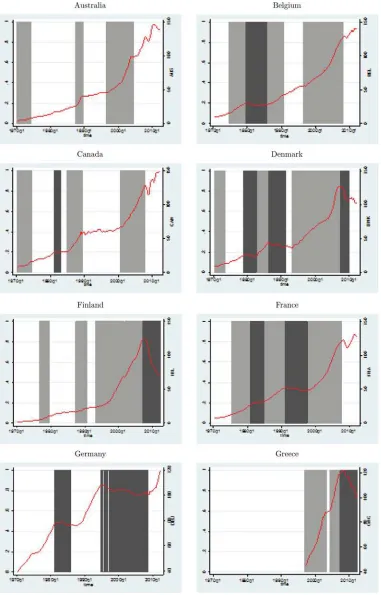
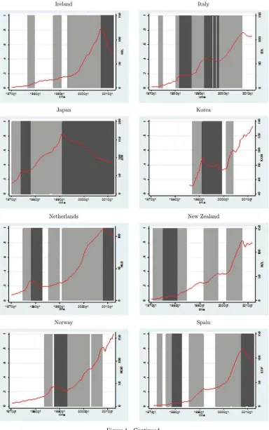
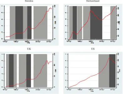
pre-vious section—we are able to identify 59 booms, 31 busts, and 59 normal time spells.Figure 1shows the booms (light shaded areas) and the busts (dark shaded regions) as compared with the normal periods (nonshaded areas) over time and across coun-tries. It is worth noting that, with the exceptions of Australia and Germany, all the other countries have experienced booms and busts and, in most of the cases, boom–bust cycles. In particular, a large group of countries including Denmark, France, Italy, Swe-den, and the U.K. could be labeled as “repeated boom busters.” Another group of countries can be labeled as “new busters,” as they were hardly hit by the subprime mortgage crisis. While this was initially confined to the U.S., it quickly spilled over the European housing markets, in particular, in countries such as Greece, Ireland, the Netherlands, and Spain, which recorded the most severe bust episodes in the Summer of 2007 and the beginning of 2008. The recent drawn-out bust seems to be rel-atively muted only in Belgium, Norway, and Switzerland (the “resilient league”). Finally, Australia and Canada can be called as “boomers” given that the periods of boom in their housing markets have never been followed by sharp collapses in housing prices. Despite this, it is important to highlight that the limited number of housing booms and housing busts makes the esti-mation of the duration models unfeasible on a country basis. Consequently, we implement the econometric framework on a panel structure.
While testing for the presence of duration dependence in housing price phases and change-points in their behavior, we also allow for differences between European and non-European countries. That is, we test whether there is a significant differ-ence in the average duration of housing price phases, as well as in the duration dependence parameter,p, between these two groups of countries. This is done by including the dummy D EC in the model, which takes the value of 1 for European countries and 0 otherwise. Additionally, we estimate separate regressions for each of these groups.
We also take into account the effects of some regressors that are assumed to be time-invariant. For the analysis of the busi-ness cycle, Zellner (1990) and Sichel (1991) suggested that the duration of the previous business cycle phase may affect the length of the current phase. Therefore, we assess whether that might also be the case for housing market cycles and include the variable DurPrev in the estimations. The type of the previ-ous phase is also controlled for with the dummy variable Prev: during booms, this dummy variable takes value 1 for busts and 0 for normal times; during busts, it takes value 1 for booms and 0 for normal times; and during normal times, it takes value 1 for booms and 0 for busts.
In addition, we analyze whether the duration of booms, busts, and normal times becomes gradually longer or shorter over time. As such, we consider a trend variable, labeled as Event, which reports the order or the observation number of each event over time and for every single country: it is equal to 1 for the first event, 2 for the second one, and so on. If the coefficient asso-ciated to this variable is significantly smaller (larger) than zero,
phase durations get longer (shorter) over time. Additionally, we replace this variable by a set of dummy variables correspond-ing to the four decades involved in the analysis: Dec70, Dec80, Dec90, Dec00.
InTable 1, we report the descriptive statistics regarding the duration of the housing price episodes. It shows the number of spells for each type of episode (Obs) and for all countries (All), for European countries (EC) and for non-European countries (NEC). It can be seen that, on average, booms and busts last the same time, but normal times tend to be slightly shorter. Interest-ingly, housing booms seem to last longer for European countries than for non-European countries, but the opposite happens for busts and normal times. Whether these differences are statisti-cally significant or not is an issue that we will try to answer with the estimation of the continuous-time Weibull model.
4.2 The Baseline Model
The empirical evidence that emerges from the estimation of the Weibull model presented in Section3.2is summarized in Table 2. A one-sided test is used to detect the presence of positive duration dependence (i.e., whether p >1) and the sign “+” indicates significance at a 5% level. The results corroborate such hypothesis for housing booms and busts, that is, the likelihood of the end of a boom or a bust phase in the housing market increases as the time goes by. This is valid not only for the basic regressions presented in Column 1, but also for the other regressions. Moreover, in most of the cases, p is equal to 2, that is, the statistical analysis of the second-order derivative of the baseline hazard function indicates the presence of constant positive duration dependence both in booms and busts. This means that the probability of booms and busts ending at timet, given that they lasted until that moment, increases over time at a constant rate. For details on the analysis of the second-order derivative of the baseline hazard function, see Castro (2010, 2013).
While we start by assuming that housing booms and busts may last from one quarter to the maximum number of time periods that are observable in our sample, the data suggest that their minimum duration is five and seven quarters, respectively. Therefore, we investigate if truncating those phases at their minimum duration affects the results or not. This implies that the hazard rate must be zero for the first quarter and some nonzero value thereafter. Truncation is set at the minimum observable duration for housing booms and busts, that is:d0=min(di)−1,
where min(di) is the shortest boom/bust observed in the sample.
As a result, the survival function becomes
S(ti,xi)=exp−γ(t
Column 2 ofTable 2displays the results where we allow for truncation and shows the main findings are not affected, that is, there is still positive duration dependence in housing booms and busts. In general, the results in this type of studies are not sensitive to the choice of the minimum observable duration (Sichel1991; Castro2010,2013).
In the regressions presented in Column 1, the population of individual spells is assumed to be homogeneous, as each housing boom or bust is under the same risk of ending. Given that this may not be a good description of reality, Column 3
Figure 1. Real housing prices, booms, busts, and normal times.Note: Booms and busts episodes are identified using the methodology proposed by Burnside et al. (2011). Dark shaded areas denote bust phases while light shaded regions indicate boom phases. The vertical axis denotes the index. The horizontal axis corresponds to time.
allows for the presence of unobserved heterogeneity or frailty. In statistical terms, a frailty model is similar to a random-effects model for duration analysis: it represents an unobserved random proportionality factor that modifies the hazard function of an individual spell and accounts for the heterogeneity caused by
unmeasured covariates or measurement errors. To include frailty in the Weibull model, the hazard function expressed by Equation (7) is modified as follows:
h(t,x|v)=vh(t,x), (21)
Figure 1. Continued.
wherevis an unobserved individual-spell effect that scales the no-frailty component. The random variablevis assumed to be positive with unity mean, finite variance,θ, and independently distributed fromtandx. The survival function is then expressed as
S(t,x|v)=[S(t,x)]v. (22)
Since the values ofvare not observed, we cannot estimate them. In this context, we follow Lancaster (1990) and assume thatvfollows a Gamma distribution with unity mean and vari-anceθ, implying that the frailty survival function can be written as
S(t,x|β, θ)=[1−θlnS(t,x)]−(1/θ), (23)
Figure 1. Continued.
while the frailty hazard function becomes
h(t,x|β, θ)=h(t,x) [S(t,x|β, θ)]θ, (24)
and the corresponding log-likelihood function can be expressed as
lnL(·)= n
i=1
ci[lnγ+lnp+(p−1) lnti+β′xi]
−
ci+
1
θ
ln
1+γ tipexp(β′xi)
. (25)
The variance parameter,θ, which measures the presence (or absence) of unobserved heterogeneity, needs to be estimated. Asθ is always greater than zero, the limiting distribution of its maximum-likelihood estimate is a normal distribution that is halved or chopped-off at the zero-bound. Therefore, the
like-lihood ratio test, LR test, that is used to detect its presence is a “boundary” test that takes into account the fact that the null distribution is not the usual chi-squared with one degree of freedom, but rather a mixture of a chi-squared with zero de-grees of freedom and a chi-squared with one degree of freedom (Gutierrez et al.2001). The results do not show strong evidence of unobserved heterogeneity, as corroborated by thep-value of the LR test reported at the bottom of Column 3: at a 5% sig-nificance level, we reject the presence of frailty. Despite this, some works emphasize the cross-country heterogeneity, even among the European countries. For instance, Carstensen et al. (2009) showed that transmission of monetary policy shocks to macroeconomic variables is amplified in the case of countries with a stronger response of real house prices. Berben et al. (2004) highlighted that the financial structures, the fiscal pol-icy framework, and the credit channel contribute to account
Table 1. Descriptive statistics
Booms Busts Normal Times
Dur Obs. Mean S.D. Min. Max. Obs. Mean S.D. Min. Max. Obs. Mean S.D. Min. Max.
All 59 23.5 14.2 6 68 31 23.1 14.6 8 85 59 18.6 17.1 2 107
EC 44 23.9 15.0 6 68 25 21.2 9.3 10 55 44 15.3 11.2 2 54
NEC 15 22.6 11.7 9 53 6 31.2 27.6 8 85 15 28.3 26.2 2 107
D EC 59 0.75 0.44 0 1 31 0.81 0.40 0 1 59 0.75 0.44 0 1
Event 59 2.19 1.06 1 5 31 1.42 0.56 1 3 59 2.20 1.06 1 5
Prev 53 0.25 0.43 0 1 31 0.84 0.37 0 1 44 0.73 0.45 0 1
DurPrev 53 18.4 17.1 2 107 31 25.2 16.5 4 68 44 22.5 12.3 7 55
NOTE: Booms and busts episodes are identified using the methodology proposed by Burnside et al. (2011). The table reports the number of episodes (Obs.), the mean duration (Mean), the standard deviation (S.D.), the minimum (Min.) and the maximum (Max.) duration for each spell. The data are quarterly and comprises 20 industrialized countries over the period 1970Q1–2012Q2.
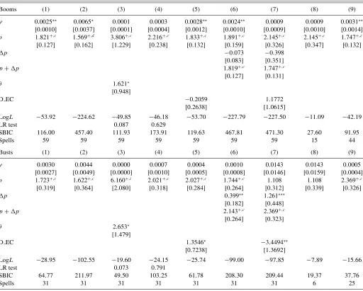
Table 2. Duration dependence in housing booms and busts: Basic Weibull model estimations
Booms (1) (2) (3) (4) (5) (6) (7) (8) (9)
γ 0.0025∗∗ 0.0065∗ 0.0001 0.0003 0.0028∗∗ 0.0024∗∗ 0.0009 0.0009 0.0031∗∗
[0.0010] [0.0037] [0.0001] [0.0004] [0.0012] [0.0010] [0.0009] [0.0010] [0.0014]
p 1.821+,c 1.569+,d 3.806+,c 2.216+,c 1.833+,c 1.891+,c 2.145+,c 2.145+,c 1.747+,c [0.127] [0.162] [1.229] [0.238] [0.132] [0.159] [0.326] [0.347] [0.132]
p −0.073 −0.398
[0.083] [0.351]
p+p 1.819+,c 1.747+,c
[0.127] [0.131]
θ 1.621∗
[0.948]
D EC −0.2059 1.1772
[0.2638] [1.0615]
LogL −53.92 −224.62 −49.85 −46.18 −53.70 −227.79 −227.50 −11.09 −42.19
LR test 0.087 0.629
SBIC 116.00 457.40 111.93 173.91 119.63 467.81 471.30 27.60 91.95
Spells 59 59 59 59 59 59 59 15 44
Busts (1) (2) (3) (4) (5) (6) (7) (8) (9)
γ 0.0030 0.0044 0.0000 0.0007 0.0004 0.0010 0.0143 0.0143 0.0005 [0.0027] [0.0049] [0.0000] [0.0010] [0.0005] [0.0008] [0.0146] [0.0159] [0.0004]
p 1.723+,c 1.622+,c 6.160+,i 2.021+,c 2.027+,c 1.744+,c 1.108 1.108 2.369+,c [0.319] [0.364] [2.080] [0.318] [0.284] [0.264] [0.312] [0.339] [0.326]
p 0.399∗∗ 1.261∗∗∗
[0.182] [0.448]
p+p 2.143+,c 2.369+,c
[0.264] [0.323]
θ 2.653∗
[1.479]
D EC 1.3546∗ −3.4494∗∗
[0.7238] [1.3692]
LogL −28.95 −102.55 −19.60 −24.15 −25.74 −99.00 −97.85 −7.89 −15.66
LR test 0.073 0.791
SBIC 64.77 211.97 49.50 103.25 61.78 208.30 209.44 19.37 37.76
Spells 31 31 31 31 31 31 31 6 25
NOTE: Heteroscedasticity and serial autocorrelation robust standard errors clustered by country are reported in square brackets;+indicates thatpis significantly higher than 1 using a one-sided test with a 5% significance level;d,c, andiindicate decreasing, constant and increasing positive duration dependence, respectively;△pis the estimated difference in the duration dependence parameter between European and Non-European countries; hence,p+pis the value of the duration dependence parameter for the European countries;∗∗∗,∗∗, ∗—statistically significant at 1%, 5%,and 10% level, respectively. Truncation at the minimum values of Dur is used in the regressions presented in Column 2. In Column 3, thep-value of the LR test for unobserved heterogeneity/frailty gives assesses if the estimated variance (θ) is different from zero. In Column 4, thep-value of the LR test analyses the statistical significance of country-specific dummy variables (pooling test), that is, LR= −2(logLr−logLu), whereranducorrespond to the restricted and unrestricted models, respectively.
Columns 8 and 9 present separate regression results for the non-European and European countries, respectively. The Schwartz Bayesian information criterion (SBIC) is computed as follows: SBIC=2(−logL+(k/2)logN), wherekis the number of regressors andNis the number of observations (spells).
for the heterogeneity in the responses of countries to a mon-etary policy shock. Additionally, while entry barriers and per-vasiveness of the employment protection legislation raise the adjustment costs associated with a monetary policy shock, the industrial structure does not seem to play an important role. Georgiadis (2012) found that a large share of the cross-country asymmetries in the response of output and prices to a mone-tary policy shock is explained by cross-country differences in the financial structure, the industry mix, and the labor market rigidity.
Even though the presence of frailty is not statistically sig-nificant, individual-country effects may still be present, given that the sample consists of 20 countries that can have individual-specific characteristics. Therefore, in Column 4, we add country-dummy variables to the set of regressors. In this case, we test for
pooling, that is, the LR test is used to assess whether the model controlling for country-specific effects is preferred to simple pooling. Thep-value of the LR test reported at the bottom of Column 4 does not support the existence of country-specific effects. Hence, we are unable to find heterogeneity in the popu-lation of individual boom and bust spells.
In Column 5, we analyze if the mean duration of housing booms and busts is significantly different for European and non-European countries, by adding the dummy variable D EC to the set of regressors. We find that the coefficient associated to D EC is not statistically significant for booms, but remains marginally significant (and positive) for busts. This suggests that, on average, housing booms tend to last the same in Eu-ropean and non-EuEu-ropean countries, while busts are shorter for European countries. Indeed, a positive coefficient implies a
higher probability of the event ending over time, that is, a shorter duration.
One question remains: is the duration dependence parameter the same for European and non-European countries in the re-spective housing phase? To answer it, we start by replacing the parameterpbyp+pin Columns 7 and 8; in Column 8, we also include the dummy variable D EC. The empirical findings confirm that the average duration of booms in European and non-European countries is broadly the same and constant posi-tive duration dependence characterizes housing booms in both groups of countries. However, with regard to housing busts, the results show that there are significant differences in the magni-tude of the duration dependence parameter and in the average duration of busts in European and non-European countries. In particular, housing busts are not duration-dependent in non-European countries, but still display constant positive duration dependence in European countries.
Finally, in Columns 8 and 9, we estimate separate regressions for non-European and European countries, respectively. The re-sults confirm that the duration dependence parameter is very similar for housing booms and there is constant positive dura-tion dependence for both groups. They also reveal that housing busts are not duration-dependent for non-European countries, while positive duration dependence characterizes housing busts in European countries.
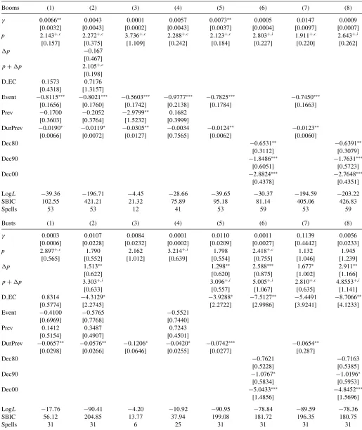
As we are using a continuous-time duration model, there is no scope to add regressors that are time-variant, but it is possible to consider some that remain constant over each spell, such as the dummy variable D EC. Other regressors include the trend variable Event, the previous phase, Prev, and the duration of the previous phase, DurPrev. In Column 1 ofTable 3, we consider these additional regressors. The empirical findings confirm the presence of constant positive duration dependence in housing booms and housing busts. Moreover, they show that booms have become longer over time, as the coefficient on Event is negative, which means that the likelihood of a boom ending fell over time. In addition, the longer the previous phase is, (no matter what, as the coefficient on Prev is not statistically significant), the smaller the likelihood of a housing boom ending tends to be, that is, housing booms typically last longer. In the case of housing busts, we find that the longer the previous phase is, the longer the housing bust will be.
In Column 2, we investigate whether the inclusion of these time-invariant regressors affects the conclusions regarding the differences in the duration dependence parameter between Eu-ropean and non-EuEu-ropean countries. As before, we show that it is not statistically different for the two groups of countries and uncover the presence of constant positive duration depen-dence. Moreover, the variable Event and DurPrev are statis-tically significant. In what concerns housing busts, the dura-tion dependence parameter is significantly larger for European countries and we only find evidence of positive duration depen-dence for this group. We reach the same conclusions when we estimate separate regressions for non-European and European countries (Columns 3 and 4). Due to the small number of busts for the non-European countries, we only include the regressor that presented a significant coefficient (DurPrev). Moreover, it also remains significant for the group of European countries.
Regarding the housing booms in the non-European countries, we should stress that the likelihood of their end decreases with the duration of the previous phase, especially if it was a bust (Prev has a significantly negative coefficient).
In Column 5, we only include the regressors with significant coefficients and find the same empirical evidence. These regres-sors are then excluded in the regressions presented in Column 6 and replaced by dummies for the decades. While these are measures of the passage of time like Event, they are based on a real-time perspective and not on a sequence or order of events over time. The results are quite interesting because: (i) they con-firm the trend toward a fall in the likelihood of housing booms ending over time; and (ii) they unveil a similar feature for hous-ing busts, which was not captured by the variable Event. This means that, over the last decades, the boom–bust cycles have become longer. These results may be linked with the works that argue that the pre-Volcker period is characterized by in-determinacy (Lubik and Schorfheide2004; Beyer and Farmer 2007; Bullard and Singh2008). Other authors also suggested that there may be a change in the monetary policy regime be-fore and after the 1980s (Schmitt-Grohe et al.2001; Benhabib et al.2002; Sargent et al.2006). In addition, Stock and Wat-son (2005), among others, identified a “structural change” in the business cycle dynamics even among the major industri-alized countries. Consequently, our empirical findings seem to indicate that such regime changes in the monetary policy and in the real economic activity that took place in the 1980s have contributed to longer housing cycles since then, as indicated by the negative and significant coefficients for the respective decades.
Additionally, in the case of housing busts, we continue to ob-serve significant differences regarding the duration dependence parameter and the respective mean durations between European and non-European countries.
Finally, Columns 7 and 8 present the same specifications as Columns 5 and 6, respectively, but with the truncation set at the minimum duration, that is, six quarters in the case of housing booms and eight quarters for housing busts. The main conclusions are not significantly affected with this change.
InTable 4, we apply the same kind of analysis to the “normal times.” The results indicate that positive duration dependence is only found when additional regressors are included in the model and, in particular, for European countries. We also find that: (i) setting truncation at the minimum duration of normal times (i.e., two quarters) does not affect the magnitude of the duration dependence parameter,p(Column 2); (ii) “frailty” effects and fixed effects are not present (Columns 3 and 4, respectively); (iii) normal times are typically shorter in European countries (Columns 5, 10, 11, 14, and 15); (iv) the duration dependence parameter is higher for European countries (Columns 6–13); (v) the likelihood of “normal times” ending is negatively affected by the duration of the previous phase, no matter what its type is (Columns 10, 11, and 14); and (vi) the duration of normal times has increased over time (Column 15), which, together with the findings for housing booms and housing busts, shows an increase in the persistence of the housing price phases and, consequently, a substantial increase in the length of the housing market cycles over time.
Table 3. Duration dependence in housing booms and busts: Basic Weibull model with additional regressors
Booms (1) (2) (3) (4) (5) (6) (7) (8)
γ 0.0066∗∗ 0.0043 0.0001 0.0057 0.0073∗∗ 0.0005 0.0147 0.0009
[0.0032] [0.0043] [0.0002] [0.0043] [0.0037] [0.0004] [0.0097] [0.0007]
p 2.143+,c 2.272+,c 3.736+,c 2.288+,c 2.123+,c 2.803+,i 1.911+,c 2.643+,i [0.157] [0.375] [1.109] [0.242] [0.184] [0.227] [0.220] [0.262]
p −0.167
[0.467]
p+p 2.105+,c [0.198]
D EC 0.1573 0.7176
[0.4318] [1.3157]
Event −0.8115∗∗∗ −0.8021∗∗∗ −0.5603∗∗∗ −0.9777∗∗∗ −0.7825∗∗∗ −0.7450∗∗∗
[0.1656] [0.1760] [0.1742] [0.2138] [0.1784] [0.1663] Prev −0.1700 −0.2052 −2.9799∗∗ 0.1682
[0.3603] [0.3764] [1.5232] [0.3999]
DurPrev −0.0190∗ −0.0119∗ −0.0305∗∗ −0.0034 −0.0124∗∗ −0.0123∗∗
[0.0066] [0.0072] [0.0127] [0.7565] [0.0062] [0.0060]
Dec80 −0.6531∗∗ −0.6391∗∗
[0.3112] [0.3079]
Dec90 −1.8486∗∗∗ −1.7631∗∗∗
[0.6051] [0.5723]
Dec00 −2.8824∗∗∗ −2.7648∗∗∗
[0.4378] [0.4351]
LogL −39.36 −196.71 −4.45 −28.66 −39.65 −30.37 −194.59 −203.22
SBIC 102.55 421.21 21.32 75.89 95.18 81.14 405.06 426.83
Spells 53 53 12 41 53 59 53 59
Busts (1) (2) (3) (4) (5) (6) (7) (8)
γ 0.0003 0.0107 0.0084 0.0001 0.0110 0.0011 0.1139 0.0056 [0.0006] [0.0228] [0.0232] [0.0002] [0.0209] [0.0027] [0.4442] [0.0233]
p 2.897+,c 1.790 2.162 3.214+,i 1.798 2.418+,c 1.132 1.945 [0.565] [0.552] [1.012] [0.639] [0.554] [0.755] [1.046] [1.239]
p 1.513∗∗ 1.298∗∗ 2.588∗∗∗ 1.677∗ 2.911∗∗
[0.622] [0.620] [0.875] [1.002] [1.166]
p+p 3.303+,i 3.096+,i 5.005+,i 2.810+,c 4.8553+,i
[0.633] [0.557] [1.067] [0.635] [1.141]
D EC 0.8314 −4.3129∗ −3.9288∗ −7.5127∗∗ −5.4491 −8.7066∗∗
[0.5774] [2.2745] [2.2722] [2.9986] [3.9241] [4.1233]
Event −0.4100 −0.5765 −0.5521
[0.6969] [0.7768] [0.7440]
Prev 0.1412 0.3487 0.7243
[0.5154] [0.4907] [0.4501]
DurPrev −0.0657∗∗ −0.0576∗∗ −0.1206∗ −0.0420∗ −0.0742∗∗∗ −0.0654∗∗
[0.0298] [0.0266] [0.0646] [0.0255] [0.0277] [0.287]
Dec80 −0.7621 −0.7163
[0.5228] [0.5385]
Dec90 −1.0767∗ −1.0196∗
[0.5834] [0.5953]
Dec00 −5.0433∗∗∗ −4.8452∗∗∗
[1.4856] [1.5696]
LogL −17.76 −90.41 −4.20 −10.92 −90.95 −78.84 −89.59 −78.36
SBIC 56.12 204.85 13.77 37.94 199.08 181.72 196.35 180.75
Spells 31 31 6 25 31 31 31 31
NOTE: SeeTable 2. Columns 3 and 4 present separate regression results for the non-European and European countries, respectively. Truncation at the minimum values of Dur is used in the regressions presented in Columns 7 and 8.
Table 4. Duration dependence in normal times: Basic Weibull model estimations
Normal (1) (2) (3) (4) (5) (6) (7) (8) (9) (10) (11) (12) (13) (14) (15)
γ 0.0241∗∗ 0.0356∗ 0.0143∗∗ 0.0019 0.0093 0.0174∗∗ 0.0182 0.0182 0.0171∗ 0.0120 0.0043 0.0007 0.0368 0.0071 0.0429∗∗
[0.0101] [0.0189] [0.0073] [0.0019] [0.0061] [0.0082] [0.0145] [0.0158] [0.0099] [0.0108] [0.0061] [0.0008] [0.0350] [0.0045] [0.0183]
p 1.181 1.176 1.447+,d 1.613+,d 1.297+,d 1.130 1.119 1.119 1.375+,d 1.581+,d 1.141 1.454 1.506+,d 1.590+,d 1.229+,d
[0.130] [0.155] [0.255] [0.196] [0.137] [0.132] [0.190] [0.185] [0.182] [0.195] [0.295] [0.886] [0.199] [0.163] [0.117]
p 0.240∗∗ 0.256 −0.365
[0.101] [0.262] [0.312]
p+p 1.370+,d 1.375+,d 1.506+, d
[0.152] [0.180] [0.203]
θ 0.412
[0.461]
D EC 0.8526∗∗ −0.0639 0.9863∗∗∗ 2.2244∗ 1.0990∗∗∗
[0.4206] [0.9825] [0.3555] [1.2003] [0.3461]
Event −0.0610 −0.5589 0.2945 −0.0897
[0.2066] [0.2122] [0.4938] [0.2139]
Prev −0.3691 −0.3879 −5.6961∗∗∗ −0.0663
[0.4589] [0.4454] [1.9747] [0.4082]
DurPrev −0.0353∗ −0.0351∗ −0.0108 −0.0368∗ −0.0353∗∗
[0.0189] [0.0189] [0.0435] [0.0198] [0.0163]
Dec80 −0.6432∗∗
[0.2875]
Dec90 −0.8940∗∗
[0.4546]
Dec00 −1.2570∗∗∗
[0.2943]
LogL −77.08 −195.45 −76.30 −64.96 −73.80 −193.53 −193.53 −20.45 −53.01 −45.22 −127.39 −5.53 −33.60 −45.68 −72.68 LR test 0.372 0.113
SBIC 162.32 399.06 164.84 207.40 159.82 399.30 403.37 46.31 113.59 113.15 281.28 18.52 84.52 106.50 165.74
Spells 59 59 59 59 59 59 59 15 44 44 44 12 32 44 59
NOTE: See Tables2and3. Truncation at the minimum values of Dur is used in the regression presented in Column 2. In Column 3, thep-value of the LR test for unobserved heterogeneity/frailty assesses whether the estimated variance (θ) is different from zero or not. In Column 4, thep-value of the LR test analyses the statistical significance of country-specific dummy variables (pooling test), that is, LR= −2(logLr−logLu), whereranducorrespond to the restricted and unrestricted models,
respectively. Columns 8, 12, and 9, 13 present separate regression results for the non-European and European countries, respectively.
4.3 The Model With Change-Points in Duration Dependence
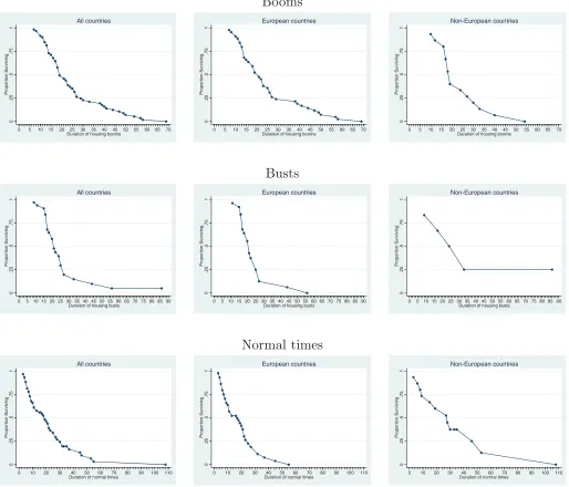
The results presented so far rely on the assumption that the magnitude of duration dependence parameter is time-invariant. To have a first idea of the plausibility of such hypothesis, in Fig-ure 2, we plot the survivor functions for housing booms, busts, and normal times for all countries, European and non-European countries. It shows that the proportion of booms, busts, or nor-mal times surviving after durationti substantially decreases as
they become older. This sharp decline is consistent with the existence of positive duration dependence.
Moreover, for booms and busts, the survivor functions quickly fall untilti =26 (for the full sample and and the European), or
ti =18 (in the case of housing booms in non-European
coun-tries). Then, they evolve at a slower pace. This, in turn, suggests
the possibility of a break in the duration dependence and the need of a more flexible framework allowing for a change-point in the Weibull distribution atτc=26 (orτc=18). Indeed, the
figure points to a duration dependence parameter that might be lower when housing booms and busts are longer than 26 quarters (18 quarters for non-European countries) and to the possibility that the likelihood of their ending significantly changes above that period.
Another signal of the existence of a break-point in duration dependence for booms and busts is provided by the slope of the survivor functions. In the case of the full sample, the av-erage slope is equal to−0.0400 (−0.0701) for housing booms (busts) that are shorter than 26 quarters and−0.0176 (−0.0368) for those that last longer than 26 quarters. Putting it differ-ently, when housing booms (busts) have a duration shorter than 26 quarters, each additional quarter of duration, on average,
0
Figure 2. Survivor functions: Booms, busts, and normal times in the housing market.
Table 5. Duration dependence in housing booms and busts: Weibull model estimations with change-points
Booms (1) (2) (3) (4) (5) (6) (7) (8)
γ1 0.0427∗∗∗ 0.0778∗∗∗ 0.1967 0.1066∗∗∗ 0.0841 0.0769∗∗∗ 0.1858∗∗∗ 0.1349 [0.0017] [0.0100] [0.6499] [0.0292] [0.0652] [0.0249] [0.0495] [0.0220]
γ2 0.0489∗∗∗ 0.1727∗∗ 0.4221 0.2710 0.2012 0.1294 0.9436 0.3270∗∗ [0.0060] [0.0732] [2.7037] [0.3012] [0.2446] [0.1108] [0.6917] [0.1606]
p1 2.611+,i 3.021+,i 4.942+,i 2.969+,i 2.984+,i 3.495+,i 2.795+,i 3.333+,i [0.310] [0.375] [2.340] [0.344] [0.394] [0.434] [0.473] [0.495]
p2 1.140 1.416 3.081+,c 1.551 1.410 1.998+,c 1.376 1.954+,c [0.155] [0.264] [1.144] [0.415] [0.261] [0.362] [0.294] [0.393]
p2−p1 −1.472∗∗∗ −1.605∗∗∗ −1.860 −1.419∗∗ −1.574∗∗∗ −1.498∗∗ −1.419∗∗ −1.378∗∗ [0.395] [0.542] [2.447] [0.595] [0.533] [0.641] [0.642] [0.703]
D EC 0.1188
[0.3710]
Event −0.7976∗∗∗ −0.5118∗∗∗ −0.9028∗∗∗ −0.7751∗∗∗ −0.7549∗∗∗
[0.1470] [0.1779] [0.2017] [0.1548] [0.1534]
Prev −0.2495 −2.4662 0.0142
[0.3447] [1.650] [0.4428]
DurPrev −0.0141∗∗ −0.0264∗∗ −0.0076 −0.0148∗∗ −0.0145∗∗
[0.0063] [0.0127] [0.0227] [0.0058] [0.0059]
Dec80 −0.8091∗∗ −0.7806∗∗
[0.3614] [0.3591]
Dec90 −1.7751∗∗∗ −1.7221∗∗∗
[0.5461] [0.5316]
Dec00 −2.7052∗∗∗ −2.6331∗∗∗
[0.4175] [0.4176]
LogL −222.57 −192.22 −40.79 −146.81 −192.62 −201.60 −191.76 −200.92
SBIC 451.15 412.24 98.98 319.61 409.07 431.75 403.37 426.31
Spells 59 53 12 41 53 59 53 59
Busts (1) (2) (3) (4) (5) (6) (7) (8)
γ1 0.0436∗∗∗ 0.0653∗ 0.0342∗∗∗ 0.0602∗∗∗ 0.0703∗∗∗ 0.1177 0.0317 [0.0021] [0.0377] [0.0028] [0.0125] [0.0053] [0.0734] [0.0312]
γ2 0.0962 0.3456 0.0222∗ 0.2460∗∗∗ 0.1826 0.4202∗∗ 0.8421 [0.0690] [1.1208] [0.0116] [0.0896] [0.1339] [0.1798] [0.6743]
p1 3.930+,i 4.342+,i 4.844+,i 4.258+,i 4.588+,i 4.103+,i 4.552+,i
[0.617] [0.825] [0.906] [0.800] [0.829] [0.887] [0.861]
p2 0.541 1.047 1.042 1.028 1.779 0.977 1.780
[0.287] [0.517] [0.485] [0.415] [0.851] [0.530] [0.854]
p2−p1 −3.389∗∗∗ −3.295∗∗∗ −3.802∗∗∗ −3.229∗∗∗ −2.810∗∗∗ −3.125∗∗∗ −2.772∗∗∗
[0.706] [0.809] [0.785] [0.851] [1.019] [0.975] [1.0406]
D EC 0.5341
[0.5818]
Event −0.1135 −0.1428
[0.6487] [0.7088]
Prev −0.2022 0.1367
[0.4833] [0.3109]
DurPrev −0.0474∗∗ −0.0386∗ −0.0526∗∗ −0.0510∗∗
[0.0231] [0.0226] [0.0240] [0.0252]
Dec80 −0.8066∗ −0.8002
[0.4908] [0.4919]
Dec90 −1.2413∗∗ −1.2336∗∗
[0.5834] [0.5849]
Dec00 −3.5881∗∗∗ −3.5801∗∗∗
[1.1541] [1.1586]
LogL −91.70 −86.67 −68.98 −87.28 −82.15 −87.02 −81.11
SBIC 193.71 200.81 160.49 191.73 184.90 187.78 184.82
Spells 31 31 25 31 31 31 31
NOTE: See Tables2and3.p2−p1is the estimated difference in the duration dependence parameters. Columns 3 and 4 present separate regression results for the non-European and
European countries, respectively. The change-point is located at duration equal to 26 quarters for booms (18 for non-European countries - Column 3) as well as for busts (due to the small number of observations, the analysis is not feasible for non-European countries). Truncation at the minimum values of Dur is used in the regressions presented in Columns 7 and 8.
increases the likelihood of their end by 4.00 (7.01) percent-age points, respectively. In contrast, in the case of longer booms (boosts), each additional quarter of duration raises the likelihood of their end by just 1.76 (3.68) percentage points, respectively. Similar results can be found for the sample of European and non-European countries: (i) in the case of non-European countries, the average slope of the survivor function changes from−0.0447 to−0.0238 for booms and from−0.0928 to−0.0622 for busts; and (ii) for non-European countries, the average slope of the survivor function changes from−0.1067 (in the case of booms that are shorter than 18 quarters) to −0.0667 (for booms that are longer than 18 quarters).
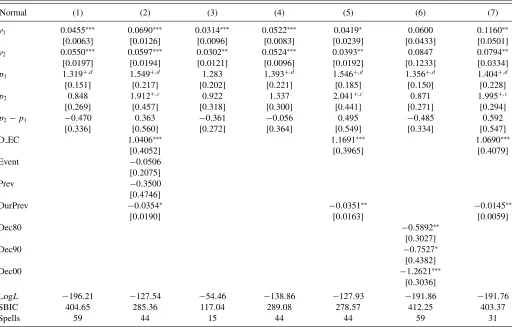
Regarding the survivor functions for normal times and fol-lowing the graphical analysis indicating at most a slight change in their slope, we consider the following durations for potential change-points: 31, for all countries; 21, in the case of European countries; and 29 for non-European countries. The differences in the slopes before and after the change-points are not substantial. Indeed, our computations show that they change: from−0.0335 to−0.0243 for the full sample; from−0.0423 to−0.0430 for the European countries; and from−0.0698 to−0.0750 for the non-European countries.
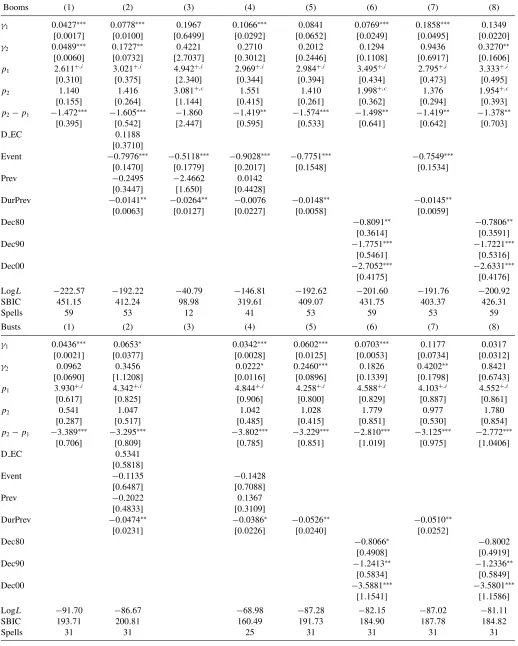
To test for the presence of change-points in the duration dependence parameter, we consider a Weibull model with a
change-point. We estimate two duration dependence parame-ters, one for the first period (p1) and another one for the second period (p2), and evaluate the statistical significance of the dif-ference between the two (p2−p1). The estimates for the two constant terms areγ1=λ
p1
1 andγ2=λ
p2
2 , respectively. We use the delta method to compute the corresponding standard-errors. The results for housing booms and busts are reported in Ta-ble 5. Column 1 displays the estimates from a simple equation without covariates. In Column 2, we control for differences in the average duration of booms and busts between European and non-European countries and account for the possibility that their duration changes over time and depends on the type and the du-ration of the previous spell. Columns 3 and 4 present the results of separate regressions for non-European and European coun-tries, respectively. In Column 5, we include only the significant regressors and, in Column 6, we replace the regressors by the dummy variables for the various decades.
The results strongly suggest that the duration dependence parameter is time-varying. In fact, the magnitude of the duration dependence parameter is always significantly lower when hous-ing booms or busts are longer than 26 quarters (in the case of the full sample and the European countries) and when housing booms are longer than 18 quarters (for the non-European coun-tries). The difference between the parameters after and before
Table 6. Duration dependence in normal times: Weibull model estimations with change-points
Normal (1) (2) (3) (4) (5) (6) (7)
γ1 0.0455∗∗∗ 0.0690∗∗∗ 0.0314∗∗∗ 0.0522∗∗∗ 0.0419∗ 0.0600 0.1160∗∗ [0.0063] [0.0126] [0.0096] [0.0083] [0.0239] [0.0433] [0.0501]
γ2 0.0550∗∗∗ 0.0597∗∗∗ 0.0302∗∗ 0.0524∗∗∗ 0.0393∗∗ 0.0847 0.0794∗∗ [0.0197] [0.0194] [0.0121] [0.0096] [0.0192] [0.1233] [0.0334]
p1 1.319+,d 1.549+,d 1.283 1.393+,d 1.546+,d 1.356+,d 1.404+,d
[0.151] [0.217] [0.202] [0.221] [0.185] [0.150] [0.228]
p2 0.848 1.912+,c 0.922 1.337 2.041+,c 0.871 1.995+,c
[0.269] [0.457] [0.318] [0.300] [0.441] [0.271] [0.294]
p2−p1 −0.470 0.363 −0.361 −0.056 0.495 −0.485 0.592
[0.336] [0.560] [0.272] [0.364] [0.549] [0.334] [0.547]
D EC 1.0406∗∗∗ 1.1691∗∗∗ 1.0690∗∗∗
[0.4052] [0.3965] [0.4079]
Event −0.0506
[0.2075]
Prev −0.3500
[0.4746]
DurPrev −0.0354∗ −0.0351∗∗ −0.0145∗∗
[0.0190] [0.0163] [0.0059]
Dec80 −0.5892∗∗
[0.3027]
Dec90 −0.7527∗
[0.4382]
Dec00 −1.2621∗∗∗
[0.3036]
LogL −196.21 −127.54 −54.46 −138.86 −127.93 −191.86 −191.76
SBIC 404.65 285.36 117.04 289.08 278.57 412.25 403.37
Spells 59 44 15 44 44 59 31
NOTE: See Tables2,3,4, and5. Columns 3 and 4 present separate regression results for the non-European and European countries, respectively. The change-point is located at duration equal to 31 quarters (29 for non-European countries and 21 for European countries). Truncation at the minimum value of Dur is used in the regression presented in column 7 (convergence is not achieved when the dummies for decades are included).