M A T H E M A T I C A L
R A N D A L L B . M A D D O X
M A T H E M A T I C A L
A N D W R I T I N G
A Transition to Abstract Mathematics
T H I N K I N G
P e p p e r d i n e U n i v e r s i t y , M a l i b u , C A
A C A D E M I C P R E S S
Sponsoring Editor Barbara Holland Production Editor Amy Fleischer Marketing Coordinator Stephanie Stevens Cover/Interior Design Cat and Mouse
Cover Image Rosmi Duaso/Timepix
Copyeditor Editor’s Ink
Proofreader Phyllis Coyne et al.
Composition Interactive Composition Corporation
Printer InterCity Press, Inc.
This book is printed on acid-free paper.∞
Copyright c2002 by HARCOURT/ACADEMIC PRESS
All rights reserved.
No part of this publication may be reproduced or transmitted in any form or by any means, electronic or mechanical, including photocopy, recording, or any information storage and retrieval system, without permission in writing from the publisher.
Requests for permission to make copies of any part of the work should be mailed to:
Permissions Department, Harcourt, Inc., 6277 Sea Harbor Drive, Orlando, Florida 32887-6777.
Academic Press
A Harcourt Science and Technology Company
525 B Street, Suite 1900, San Diego, California 92101-4495, USA http://www.academicpress.com
Academic Press
Harcourt Place, 32 Jamestown Road, London NW1 7BY, UK http://www.academicpress.com
Harcourt/Academic Press
A Harcourt Science and Technology Company
200 Wheeler Road, Burlington, Massachusetts 01803, USA http://www.harcourt-ap.com
Library of Congress Control Number: 2001091290
International Standard Book Number: 0-12-464976-9
PRINTED IN THE UNITED STATES OF AMERICA
For Dean Priest
Contents
Why Read This Book
xiii
Preface
xv
CHAPTER 0
Notation and Assumptions 1
0.1 Set Terminology and Notation 1
0.2 Assumptions 5
0.2.1
Basic algebraic properties of real numbers
5
0.2.2
Ordering of real numbers
7
0.2.3
Other assumptions about
R
9
PART I
FOUNDATIONS OF LOGIC AND PROOF WRITING 11
CHAPTER 1
Logic 13
1.1 Introduction to Logic 13
1.1.1
Statements
13
1.1.2
Negation of a statement
15
1.1.3
Combining statements with AND/OR
15
1.1.4
Logical equivalence
18
1.1.5
Tautologies and contradictions
18
1.2 If-Then Statements 20
1.2.1
If-then statements
20
1.2.2
Variations on
p
→
q
22
1.3 Universal and Existential Quantifiers 27
1.3.1
The universal quantifier
27
1.3.2
The existential quantifier
29
1.3.3
Unique existence
30
1.4 Negations of Statements 31
1.4.1
Negations of
p
∧
q
and
p
∨
q
32
1.4.2
Negations of
p
→
q
33
1.4.3
Negations of statements
with
∀
and
∃
33
CHAPTER 2
Beginner-Level Proofs 38
2.1 Proofs Involving Sets 38
2.1.1
Terms involving sets
38
2.1.2
Direct proofs
41
2.1.3
Proofs by contrapositive
44
2.1.4
Proofs by contradiction
45
2.1.5
Disproving a statement
45
2.2 Indexed Families of Sets 47
2.3 Algebraic and Ordering Properties of
R
53
2.3.1
Basic algebraic properties
of real numbers
53
2.3.2
Ordering of the real numbers
56
2.3.3
Absolute value
57
2.4 The Principle of Mathematical Induction 61
2.4.1
The standard PMI
62
2.4.2
Variation of the PMI
64
2.4.3
Strong induction
65
2.5 Equivalence Relations: The Idea of Equality 68
2.5.1
Analyzing equality
68
2.5.2
Equivalence classes
72
2.6 Equality, Addition, and Multiplication in
Q
76
2.6.1
Equality in
Q
77
2.6.2
Well-defined
+
and
×
on
Q
78
2.7 The Division Algorithm and Divisibility 79
2.7.1
Even and odd integers; the division
algorithm
79
2.7.2
Divisibility in
Z
81
2.8 Roots and irrational numbers 85
2.8.1
Roots of real numbers
86
CHAPTER 3
Functions 97
3.1 Definitions and Terminology 97
3.1.1
Definition and examples
97
3.1.2
Other terminology and notation
101
3.1.3
Three important theorems
103
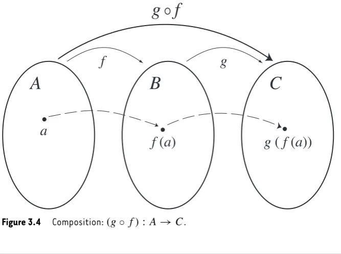
3.2 Composition and Inverse Functions 106
3.2.1
Composition of functions
106
3.2.2
Inverse functions
108
3.3 Cardinality of Sets 110
3.3.1
Finite sets
111
3.3.2
Infinite sets
113
3.4 Counting Methods and the Binomial Theorem 118
3.4.1
The product rule
118
3.4.2
Permutations
122
3.4.3
Combinations and partitions
122
3.4.4
Counting examples
125
3.4.5
The binomial theorem
126
PART II
BASIC PRINCIPLES OF ANALYSIS 131
CHAPTER 4
The Real Numbers 133
4.1 The Least Upper Bound Axiom 134
4.1.1
Least upper bounds
134
4.1.2
The Archimedean property of
R
136
4.1.3
Greatest lower bounds
137
4.1.4
The LUB and GLB properties applied
to finite sets
137
4.2 Sets in
R
140
4.2.1
Open and closed sets
140
4.2.2
Interior, exterior, and boundary
142
4.3 Limit Points and Closure of Sets 143
4.3.1
Closure of sets
144
4.4 Compactness 146
4.5 Sequences in
R
149
4.5.1
Monotone sequences
150
4.5.2
Bounded sequences
151
4.6 Convergence of Sequences 153
4.6.1
Convergence to a real number
154
4.6.2
Convergence to
±∞
158
4.7.2
The NIP applied to subsequences
162
4.7.3
From NIP to LUB axiom
164
4.8 Cauchy Sequences 165
4.8.1
Convergence of Cauchy sequences
166
4.8.2
From completeness to the NIP
168
CHAPTER 5
Functions of a Real Variable 170
5.1 Bounded and Monotone Functions 170
5.1.1
Bounded functions
170
5.1.2
Monotone functions
171
5.2 Limits and Their Basic Properties 173
5.2.1
Definition of limit
173
5.2.2
Basic theorems of limits
175
5.3 More on Limits 180
5.3.1
One-sided limits
180
5.3.2
Sequential limit of
f
181
5.4 Limits Involving Infinity 182
5.4.1
Limits at infinity
183
5.4.2
Limits of infinity
185
5.5 Continuity 187
5.5.1
Continuity at a point
188
5.5.2
Continuity on a set
190
5.5.3
One-sided continuity
194
5.6 Implications of Continuity 195
5.6.1
The intermediate value theorem
195
5.6.2
Continuity and open sets
197
5.7 Uniform Continuity 200
5.7.1
Definition and examples
200
5.7.2
Uniform continuity and compact sets
202
PART III
BASIC PRINCIPLES OF ALGEBRA 205
CHAPTER 6
Groups 207
6.1 Introduction to Groups 207
6.1.1
Basic characteristics of algebraic
structures
208
6.1.2
Groups defined
210
6.1.3
Subgroups
213
6.3 Integers Modulo
n
and Quotient Groups 220
6.3.1
Integers modulo
n
220
6.3.2
Quotient groups
223
6.3.3
Cosets and Lagrange’s theorem
225
6.4 Permutation Groups and Normal Subgroups 227
6.4.1
Permutation groups
227
6.4.2
The alternating group
A
4229
6.4.3
The dihedral group
D
8230
6.4.4
Normal subgroups
232
6.4.5
Equivalences and implications of normality
233
6.5 Group Morphisms 236
CHAPTER 7
Rings 243
7.1 Rings and Subrings 243
7.1.1
Rings defined
243
7.1.2
Examples of rings
245
7.1.3
Subrings
248
7.2 Ring Properties and Fields 249
7.2.1
Ring properties
249
7.2.2
Fields defined
254
7.3 Ring Extensions 256
7.3.1
Adjoining roots of ring elements
256
7.3.2
Polynomial rings
258
7.3.3
Degree of a polynomial
259
7.4 Ideals 260
7.4.1
Definition and examples
260
7.4.2
Generated ideals
262
7.4.3
Prime ideals
264
7.4.4
Maximal ideals
264
7.5 Integral Domains 267
7.6 UFDs and PIDs 273
7.6.1
Unique factorization domains
273
7.6.2
Principal ideal domains
274
7.7 Euclidean Domains 279
7.7.1
Definition and properties
279
7.7.2
Polynomials over a field
282
7.7.3
Z
[
t
] is a UFD
284
7.8 Ring Morphisms 287
7.8.1
Properties of ring morphisms
288
7.9 Quotient Rings 291
Why Read This Book?
One of Euclid’s geometry students asked a familiar question more than 2000 years ago. After learning the first theorem, he asked, “What shall I get by learning these things?” Euclid didn’t have the kind of answer the student was looking for, so he did what anyone would do — he got annoyed and sarcastic. The story goes that he called his slave and said, “Give him threepence since he must make gain out of what he learns.”1
It is a familiar question: “So how am I ever gonna use this stuff?” I doubt that anyone has ever come up with a good answer because it’s really the wrong question. The first question is not what you’re going to do with this stuff, but what this stuff is going to do with you.
This book is not a computer users’ manual that will make you into a computer industry millionaire. It is not a collection of tax law secrets that will save you thousands of dollars in taxes. It is not even a compilation of important mathematical results for you to stack on top of the other mathematics you have learned. Instead, it’s an entrance into a new kingdom, the world of mathematics, where you learn to think and write as the inhabitants do.
Mathematics is a discipline that requires a certain type of thinking and communi-cating that many appreciate but few develop to a great degree. Developing these skills involves dissecting the components of mathematical language, analyzing their structure, and seeing how they fit together. Once you have become comfortable with these princi-ples, then your own style of mathematical writing can begin to shine through.
Writing mathematics requires a precision that seems a little stifling because at first it might feel like some pedant is forcing you to use prechosen words and phrases to express the things you see clearly with your own mind’s eye. Be patient. In time you’ll see how adapting to the culture of mathematics and adopting its style of communicating will shape all your thinking and writing. You’ll see your skills of critical analysis become more developed and polished. My hope is that these skills will influence the way you organize 1T.L. Heath,A History of Greek Mathematics,Oxford, 1931.
and present your thoughts in everything from English composition papers to late night bull sessions with friends.
Here’s an analogy of what the first principles of this book will do for you. Consider a beginning student of the piano. Music is one of the most creative disciplines, and our piano student has been listening to Chopin for some time. She knows she has a true ear and an intuition for music. However, she must begin at the piano by playing scales over and over. These exercises develop her ability to use the piano effectively in order to express the creativity within her. Furthermore, these repetitive tasks familiarize her with the structure of music as an art form, and actually nurture and expand her capacity to express herself in original and creative ways through music. Then, once she has mastered the basic technical skills of hitting the keys, she understands more clearly how really enjoyable music can be. She learns this truth: The aesthetic elements of music cannot be fully realized until the technical skills developed by rote exercises have been mastered and can be relegated to the subconscious.
Your first steps to becoming a mathematician are a lot like those for our pianist. You will first be introduced to the building blocks of mathematical structure, then practice the precision required to communicate mathematics correctly. The drills you perform in this practice will help you see mathematics as a discipline more clearly and equip you to appreciate its beauty.
Letnbe a positive integer, and think of this course as a trip through a new country on a bicycle built forn. The purposes of the trip are:
To familiarize you with the territory; To equip you to explore it on your own;
To give you some panoramic views of the countryside; To teach you to communicate with the inhabitants; and To help you begin to carve out your own niche.
Preface
This text is written for a “transition course” in mathematics, where students learn to write proofs and communicate with a level of rigor necessary for success in their upper level mathematics courses. To achieve the primary goals of such a course, this text includes a study of the basic principles of logic, techniques of proof, and fundamental mathematical results and ideas (sets, functions, properties of real numbers), though it goes much further. It is based on two premises: The most important skill students can learn as they approach the cusp between lower- and upper-level courses is how to compose clear and accurate mathematical arguments; and they need more help in developing this skill than they would normally receive by diving into standard upper-level courses. By emphasizing how one writes mathematical prose, it is also designed to prepare students for the task of reading upper-level mathematics texts. Furthermore, it is my hope that transitioning students in this way gives them a view of the mathematical landscape and its beauty, thereby engaging them to take ownership of their pursuit of mathematics.
Why
this
text?
I believe students learn best by doing. In many mathematics courses it is difficult to find enough time for students to discover through their own efforts the mathematics we would lead them to find. However, I believe there is no other effective way for students to learn to write proofs. This text is written for them in a format that allows them to do precisely this.
Two principles of this text are fundamental to its design as a tool whereby students learn by doing. First, it does not do too much for them. Proofs are included in this text for only two reasons. Most of them (especially at the beginning) are sample proofs that students can mimic as they write their own proofs to similar theorems. Students must read them because they will need this technique later. The other proofs are included here
Second, if students are going to learn by doing, they must be presented with doable tasks. This text is designed to be a sequence of stepping stones placed just the right distance apart. Moving from one stone to the next involves writing a proof. Seeing how to step there comes from reading the exposition and calls on the experience that led the student to the current stone. At first, stones are very close together, and there is much guidance. Progressing through the text, stones become increasingly farther apart, and some of the guidance might be either relegated to a footnote or omitted altogether.
I have written this text with a very deliberate trajectory of style. It is conversational throughout, though the exposition becomes more sophisticated and succinct as students progress through the chapters.
Organization
This text is organized in the following way. Chapter 0 spells out all assumptions to be used in writing proofs. These are not necessarily standard axioms of mathematics, and they are not presented in the context or language of more abstract mathematical structures. They are designed merely to be a starting point for logical development, so that students appreciate quickly that everything we call on is either stated up front as an assumption, or proved from these assumptions. Although Chapter 0 contains much mathematical information, students can probably read it on their own as the course begins, knowing that it is there primarily as a reference.
Part I begins with logic, but does not focus on it. In Chapter 1, truth tables and manip-ulation of logical symbols are included to give students an understanding of mathematical grammar, of the underlying skeletal structure of mathematical prose, and of equivalent ways of communicating the same mathematical idea. Chapters 2 and 3 put these to use right away in proof writing, and allow the students to cut their teeth on the most basic mathematical ideas. The context of topics in Chapters 2 and 3 is often rather specific, though certainly more broadly applicable. It is designed to ground the students in famil-iar territory first, then move into generalized structures later. Abstraction is the goal, not the beginning.
and there is much flexibility in the material one may choose to cover.
First, because this text speaks directly to the student, it can naturally be used in a setting where students are given responsibility for the momentum of the class. It is written so that students can read the material on their own first, then bring to class the fruits of their work on the exercises, and present these to the instructor and each other for discussion and critique. If class time and size limit the practicality of such a student-driven approach, then certainly other approaches are possible. To illustrate, we may consider three components of a course’s activity, and arrange them in several ways. The components are: 1) the students’ reading of the material; 2) the instructor’s elaboration on the material; and 3) the students’ work on the exercises, either to be presented in class or turned in. When I teach from this text, component 1) is first, 3) follows on its heels, and 2) and 3) work in conjunction until a section is finished. Others might want to arrange these components in another order, for example, beginning with 2), then following with 1) and 3).
Which material an instructor would choose to cover will depend on the purpose of the course, personal taste, and how much time there is. Here are two broad options.
1. To proceed quickly into either analysis or algebra, first cover the material from Part I that lays the foundation. Almost all sections and exercises of Part I are necessary for Parts II and III. However, theInstructor’s Guide and Solutions Manualnotes precisely which sections, theorems, and exercises are necessary for each path, and which may be safely omitted without leaving any holes in the logical progression. Of course, even if a particular result is necessary later, one might decide that to omit its proof details does not deprive the students of a valuable learning experience. The instructor might choose simply to elaborate on how one would go about proving a certain theorem, then allow the students to use it as if they had proved it themselves.
2. Cover Part I in its entirety, saving specific analysis and algebra topics for later courses. This option might be most realistic for courses of two or three units where all the Part I topics are required. Even with this approach, there would likely be time to cover the beginnings of Parts II and/or III. This might be the preferred choice for those who do not want to study analysis or algebra with the degree of depth and breadth characteristic of this text.
This book would not have become a reality without the help of many people. First thanks go to Carolyn Vos Strache, Chair of the Natural Science Division at Pepperdine University, for providing me with resources as this project got off the ground. As it has taken shape, this project has come to bear the marks of many people whose meticulous dissection of several drafts inspired many suggestions for improvements. My thanks to colleagues at Pepperdine and from across the country for their hard work in helping shape this volume into its present form:
Irene Loomis, University of Tennessee, Chattanooga, TN Carlton J. Maxson, Texas A&M University, College Station, TX Bruce Mericle, Minnesota State University, Mankato, MN Kandasamy Muthuvel, University of Wisconsin, Oshkosh, WI Kamal Narang, University of Alaska, Anchorage, AK
Travis Thompson, Harding University, Searcy, AR Steven Williams, Brigham Young University, Provo, UT
I have written this book with the student foremost in mind. Many of my students have shaped this text from the beginning by their hard work in my class. Several students, both my own and from other universities across the country, have also made formal and useful suggestions. Their marks are indelible.
Erik Baumgarten, Texas A&M University, College Station, TX Justin Greenough, University of Alaska, Anchorage, AK Reuben Hernandez, Pepperdine University, Malibu, CA Brian Hostetler, Virginia Tech, Blacksburg, VA
Jennifer Kuske, Pepperdine University, Malibu, CA
Notation and Assumptions
S
uppose you’ve just opened a new jigsaw puzzle. What are the first things you do? First, you pour all the pieces out of the box. Then you sort through and turn them all face up, taking a quick look at each one to determine whether it’s an inside or outside piece, and you arrange them somehow so that you’ll have an idea of where certain types of pieces can be found later. You don’t study each piece in depth, nor do you start trying to fit any of them together. In short, you just lay all the pieces out on the table and briefly familiarize yourself with each one. This is the point of the game where you merely set the stage, knowing that everything you’ll need later has been put in a place where you can find it when you need it.In this introductory chapter we lay out all the pieces we will use for our work in this course. It’s essential that you read it now, in part because you need some preliminary exposure to the ideas, but mostly because you need to have spelled out precisely what you can use without proof in Part I, where this chapter will serve you as a reference. Give this chapter a casual but complete reading for now. You’ve probably seen most of the ideas before. But don’t try to remember it all, and certainly don’t expect to understand everything either. That’s not the point. Right now, we’re just organizing the pieces. The two issues we address in this chapter are: 1) set terminology and notation; and 2) assumptions about the real numbers.
0.1 Set Terminology and Notation
Sets are perhaps the most fundamental mathematical entity. Intuitively we think of a set as a collection of things, where the collection itself is thought of as a single entity. Sets may contain numbers, points in thex y-plane, functions, ice cream cones, steak knives,
Definition 0.1.1.
IfAis a set andxis an entity inA, we writex∈ A, and say thatxis anelementofA. To writex∈/ Ais to mean thatxis not an element ofA.
How can you communicate to someone what the elements of a set are? There are several ways.
1. List them. If there are only a few elements in the set, you can easily list them all. Otherwise, you might start listing the elements and hope that the reader can take the hint and figure out the pattern. For example,
(a) {1,8, π,Monday} (b) {0,1,2, . . . ,40}
(c) {. . . ,−6,−4,−2,0,2,4,6, . . .}
2. Provide a description of the criteria used to decide whether an entity is to be included. This is how it works:
(a) {x:xis a real number andx>−1}This notation should be read “the set of all xsuch thatxis a real number andxis greater than−1.” The variablexis just an arbitrary symbol chosen to represent a random element of the set, so that any characteristics it must have can be stated in terms of that symbol.
(b) {p/q : pandqare integers andq =0}This assumes you know what aninteger
is (p. 5). This is the set of all fractions, integer over integer, where it is expressly stated that the denominator cannot be zero.
(c) {x:P(x)}This is a generic form for this way of describing a set. The expression P(x)represents some specified property thatxmust have in order to be in the set. When addressing the elements of a set, or more important, when addressing all thingsnotin a particular set, we must have some universal limiting parameters in mind. Although it might not be explicitly stated, we generally consider that there is some
universal setbeyond which we do not concern ourselves. Then, if we’re talking about everything not in a setA, we know how far to cast the net. It is limited by our universal set, typically denotedU.
To help visualize sets and how they compare and combine, we sometimes sketch what is called aVenn diagram. Given a set Awithin a universal setU, we may sketch a Venn diagram as in Fig. 0.1.
Given two setsAandB, it just might happen that all elements ofAare also elements ofB. We write this asA⊆Band say thatAis asubsetofB. Equivalently, we may write
B ⊇ A, and say thatBis asuperset ofA. If Ais a subset of B, but there are elements
ofBthat are not inA, we say thatAis aproper subsetofB, and write thisA⊂B. The relationshipA⊆Bcan be displayed in the Venn diagram in Fig. 0.2. The region outside Abut insideBmay or may not have any elements.
U
A
Figure 0.1
A basic Venn diagram.
U
A
B
Figure 0.2
Venn diagram with
A
⊆
B
.
U
A
B
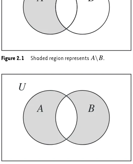
Venn diagrams are handy for visualizing new sets formed from old ones. Here are a couple of examples.
Definition 0.1.2.
Given a setA, the setA′is called thecomplementofA, and is defined as the set of all elements ofUthat are not inA(Fig. 0.4). That is,A′= {x:x∈Uandx∈/ A} (0.1)
U
A
Figure 0.4
Shaded region represents
A
′.
Definition 0.1.3.
Given two sets AandB, we define theirunion∪andintersection∩in the following way:A∪B= {x:x∈Aorx∈B} (0.2)
A∩B= {x:x∈Aandx∈B} (0.3)
An entity is allowed to be inA∪ Bprecisely when it is in at least one ofA,B. An entity is allowed to be inA∩Bprecisely when it is in bothAandB. See Figs. 0.5 and 0.6.
U
A
B
U
A
B
Figure 0.6
Shaded region represents
A
∩
B
.
Finally, we provide the notation for commonly used sets. Famous sets we need to know include the following:
Empty set:∅ = { } (the set with no elements) Natural numbers:N= {1,2,3, . . .}
Whole numbers:W= {0,1,2,3, . . .}
Integers:Z= {. . . ,−3,−2,−1,0,1,2,3, . . .}
Rational numbers:Q= {p/q : p,q ∈Z,q =0}
Real numbers:R (Explained in what follows)
0.2 Assumptions
One big question we’ll face at the outset of this course is what we are allowed to assume and what we must justify with proof. The purpose of this section is to provide a framework for the way you work with real numbers, spelling out the properties you may assume and reminding you of how to visualize them.
0.2.1 Basic algebraic properties of real numbers
The real numbersR, as well its familiar subsetsN,W,Z, and Q, are assumed to be endowed with the relation of equality and the operations of addition and multiplication, and to have the following properties. First, equality is assumed to behave in the following way:
(A1) Properties of equality:
(b) Ifa=b, thenb=a (Symmetric property);
(c) Ifa=bandb=c, thena =c (Transitive property). ■
The first property of addition we assume concerns its predictable behavior, even when the numbers involved can be addressed by more than one name. For example,3/8and 6/16are different names for the same number. We need to know that adding something to3/8will always produce the same result as adding it to6/16. The following property is our way of stating this assumption.
(A2) Addition is well defined:
That is, ifa,b,c,d ∈R, wherea =bandc=d,thena+c=b+d. ■
A special case of property A2 yields a familiar principle that goes all the way back to your first days of high school algebra: Ifa=b, then, sincec=c, we have thata+c= b+c.
(A3) Closure property of addition:
For everya,b ∈ R,a+b ∈ R. That is, the sum of two real numbers is still a real number. This closure property also holds forN,W,Z, andQ. ■
(A4) Associative property of addition:
For everya,b,c∈R,(a+b)+c=a+(b+c) ■
Addition is what we call abinary operation, meaning it combines exactly two numbers to produce a single number result. If we have three numbersa,b, andcto add up, we must split the task into two steps of adding two numbers. Property A4 says it doesn’t matter which two,aandb, orbandc, we add first. It motivates us to use the more lax notationa+b+c.
(A5) Commutative property of addition:
For everya,b∈R,a+b=b+a. ■If you’re not careful, you’ll tend to assume order does not matter when two things are combined in a binary operation. There are plenty of situations where order does matter, as we’ll see.
(A6) Existence of an additive identity:
There exists an element0∈R with theproperty thata+0=afor everya∈R. ■
(A7) Existence of additive inverses:
For everya∈R, there exists someb∈Rsuch thata+b=0. Such an elementbis called anadditive inverseofa, and is typically denoted−a to show its relationship toa. We donotassume that only one suchbexists. ■
Properties similar to A2–A7 hold for multiplication.
(A8) Multiplication is well defined:
That is, if a,b,c,d∈R, wherea = b andc=d, thenac=bd. ■
(A10) Associative property of multiplication:
For everya,b,c∈R,(a·b)·c=a·(b·c)or(ab)c=a(bc). ■
(A11) Commutative property of multiplication:
For everya,b∈R,ab=ba. ■(A12) Existence of a multiplicative identity:
There exists an element1∈Rwiththe property thata·1=afor everya ∈R. ■
(A13) Existence of multiplicative inverses:
For everya ∈ Rexcepta =0, there exists someb ∈ Rsuch that ab=1. Such an elementb is called amultiplicative inverseofaand is typically denoteda−1to show its relationship toa. As with additiveinverses, we do not assume that only one suchbexists. Furthermore, the assumption thata−1exists for alla=0does not assume that zero doesnothave a multiplicative
inverse. It says nothing about zero at all. ■
The next property describes how addition and multiplication interact.
(A14) Distributive property of multiplication over addition:
For every a,b,c∈ R,a(b+c)=(ab)+(ac)=ab+ac,where the multiplication is assumed to
be done before addition in the absence of parentheses. ■
Property A14 is important because it’s the only link between the operations of ad-dition and multiplication. Several important properties ofRowe their existence to this relationship. For example, as we’ll see later, the fact thata·0=0for everya ∈ Ris a direct result of the distributive property, and not something we simply assume.
From addition and multiplication we create the operations of subtraction and division, respectively. Knowing that additive and multiplicative inverses exist (except for0−1), we write
a−b=a+(−b) (0.4)
a/b=a·b−1 (0.5)
One very important assumption we need concerns properties A6 and A12. For rea-sons you’ll see later, we need to assume that the additive identity is different from the multiplicative identity. That is, we need the assumption
(A15)
1=0. ■We’ll use these very basic properties to derive some other familiar properties of real numbers in Chapter 2.
0.2.2 Ordering of real numbers
andnegative. Then in A17 and A18, we make some assumptions about how the positive real numbers behave.
(A16) Trichotomy law:
For anya ∈R, exactly one of the following is true: (a) a>0, in which case we sayaispositive;(b) a=0;
(c) 0>a, in which case we sayaisnegative.
■
(A17)
Ifa>0andb>0, thena+b>0. That is, the set of positive real numbersis closed under addition. ■
(A18)
Ifa >0andb>0, thenab>0. That is, the set of positive real numbers isclosed under multiplication. ■
Now we can use A16–A18 to give meaning to other statements comparing two arbi-trary real numbersaandb.
Definition 0.2.1.
Ifa,b ∈ R, we say thata > bifa−b > 0. The statementa < bmeansb > a. The statementa ≥ bmeans that eithera > bora = b. Similarly,a ≤ b
means eithera<bora=b.
The rest of the properties of real numbers are probably not as familiar as the preceding ones, but their roles in the theory of real numbers will be clarified in good time. As with the above properties, we do not try to justify them. We merely accept them and use them as a basis for proofs. A very important property of the whole numbers is the following.
(A19) Well-ordering principle:
Any nonempty subset ofW(orNfor that matter) has a smallest element. That is, ifA⊆W(orA⊆N), andAis nonempty, then there is some numbera ∈ Awith the property thata ≤xfor allx∈ A. In particular,1isthe smallest natural number. ■
The next property ofRis a bit complicated, but is indispensable in the theory of real numbers. Read it casually the first time, but know that it will be very important in Part II of this text. SupposeA⊂Ris a nonempty set with the property that it is bounded from above. That is, suppose there is someM ∈Rwith the property thata≤ Mfor alla∈ A. For example, letA= {x :x2<10
}. ClearlyM =4is a number such that everya ∈ A satisfiesa ≤M. So 4 is anupper boundfor the setA. There are other upper bounds for A, such as 10, 3.3, and 3.17. The point to be made here is that, among all upper bounds that exist for a set, there is an upper bound that is smallest, and it exists inR. This is stated in the following.
exists someM ∈Rwith the property thata ≤Mfor alla ∈ A, then there will also exist someL∈Rwith the following properties:
(L1) For everya∈ A, we have thata ≤L, and
(L2) IfNis any upper bound forA, it must be thatN ≥L. ■
0.2.3 Other assumptions about
R
The real numbers are indeed a complicated set. The final two properties ofRwe mention are not standard assumptions, and they deserve your attention at some point in your mathematical career. In this text, we assume them.
(A21)
The real numbers can be equated with the set of all base 10 decimal represen-tations. That is, every real number can be written in a form like338.1898. . ., where the decimal might or might not terminate, and might or might not fall into a pattern of repetition.Furthermore, every decimal form you can construct represents a real number. Strangely, though, there might be more than one decimal representation for a certain real number. You might remember that 0.9999. . . = 1. (See Section 2.5.1.) The repeating 9 is the only case where more than one decimal representation is possible.
We’ll assume this. ■
Our final assumption concerns the existence of roots of real numbers.
(A22)
For every positive real numberxand anyn ∈N, there exists a real number solutionyto the equationyn=x. Such a solutionyis called annth root ofx. Thecommon notation√nxwill be addressed in Section 2.8. ■
Notice we make no assumptions about how many such roots of x there are, or what their signs are. Nor do we assume anything about roots of zero or of negative real numbers. We’ll derive these from assumption A22.
P A R T
I
Logic
C H A P T E R
1
1.1 Introduction to Logic
Mathematicians make as much use of language as anyone else. Not only do they com-municate their mathematical work with language, but the use of language is itself part of the mathematical structure. In this chapter, we lay out some of the principles that govern the mathematician’s use of language.
1.1.1 Statements
The first issue we address is what kinds of sentences mathematicians use as building blocks for their work. Remember from elementary school grammar that sentences are generally divided into four classes:
Declarative sentences: We also call thesestatements. Here are some examples: 1. Labor Day is the first Monday in September.
2. Earthquakes don’t happen in California. 3. Three is greater than seven.
4. The world will end on June 6, 2040. 5. The sky is falling.
One characteristic of statements that jumps out at you is that they generally evoke a reaction such as, “Yeah, that’s true,” or “No way,” or even “Thatcouldbe true, but I don’t know for sure.” Statement 1 is true, statements 2 and 3 are false, while statements 4
its truth or falsity will be revealed. Statement 5, however, is curious. If you were going to investigate the truth or falsity of this statement, you would immediately be faced with the problem of what the terms mean. How do we define “the sky,” and what precisely does it mean to say that it “is falling”?
Imperative sentences: We would call these commands. 1. Don’t wash your red bathrobe with your white underwear. 2. Knock three times on the ceiling if you want me.
Interrogative sentences: That is, questions. 1. How much is that doggy in the window? 2. Have you always been that ugly?
Exclamations:
1. What a day!
2. Lions and tigers and bears, Oh My! 3. So, like, whatever.
The mathematician’s work centers around the first category, but we have to be care-ful about exactly which declarative sentences we allow. We will define astatement in-tuitively as a sentence that can be assigned either to the class of things we would call TRUE or to the class of things we would call FALSE. Let’s conduct a little thought experiment.
Imagine the set of all conceivable statements, and call itS. Naturally, this set is
frighteningly large and complex, but a most important characteristic of its elements is that each one can be placed into exactly one of two subsets:T(statements called TRUE),
andF(statements called FALSE). Sometimes you might have trouble recognizing whether
a sentence even belongs inS. There are, after all, things called paradoxes. For example,
“This sentence is false,” which cannot be either true or false. If you think the sentence is true, then it is false. However, if it is false, then it is true. We don’t want to allow these types of sentences inS.
Now that we have the set of all statements partitioned intoTandF, the true and
false ones, respectively, we want to look at relationships between them. Specifically, we want to pick statements fromS, change or combine them to make other statements in S, and lay out some understandings of how the truth or falsity of the chosen statements
determines the truth or falsity of the alterations and combinations. In the next part of this section, we discuss three ways of doing this:
● the negation of a statement;
1.1.2 Negation of a statement
We generally usep,q,r, and so forth, to represent statements symbolically. For example, define a statementpas follows:
p: Megan has rented a car for today.
Now consider thenegationordenialof p, which we can create by a strategic placement of the word NOT somewhere in the statement. We write it this way:
¬p: Megan has not rented a car for today.
Naturally, if pis true, then¬pis false, and vice versa. We illustrate this in atruth table(Table 1.1).
p ¬p
T F
F T
Table 1.1
Definition 1.1.1.
Given a statement p, we define the statement¬p(not p) to be false whenpis true, and true whenpis false, as illustrated in Table 1.1.1.1.3 Combining statements with AND/OR
When two statements are joined by AND or OR to produce a compound statement, we need a way of deciding whether the compound statement is true or false based on the truth or falsity of its component statements. Let’s build these with an example. Define statementspandqas follows:
p: Megan is at least 25 years old. q : Megan has a valid driver’s license. Now let’s create the statement we call “pandq,” which we write as
p∧q : Megan is at least 25 years old, and she has a valid driver’s license.
If you know the truth or falsity ofpandqindividually, how would you be inclined to categorizep∧q?1Naturally, the only way that we would considerp
p q p∧q
T T T
T F F
F T F
F F F
Table 1.2
p∧qis inTorFdepends on whetherpandqare inTorFindividually. We illustrate
the results of all different combinations in Truth Table 1.2. Notice how the truth table is constructed with four rows, systematically displaying all possible combinations ofTand
Fforpandq.
Definition 1.1.2.
Given two statementspandq, we define the statementp∧q(pandq) to be true precisely when bothpandqare true, as illustrated in Table 1.2.Now let’s join two statements with OR. Define statementspandqby p : Megan has insurance that covers her for any car she drives. q : Megan bought the optional insurance provided by the car
rental company.
The compound statement we call “porq” is written:
p∨q : Megan has insurance that covers her for any car she drives, or she bought the optional insurance provided by the car rental company.
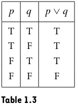
How should we assign T or F to p ∨ q based on the truth or falsity of p and q individually?2 We define p
∨q to be true ifat least one of p,q is true. See Truth Table 1.3.
p q p∨q
T T T
T F T
F T T
F F F
Table 1.3
Definition 1.1.3.
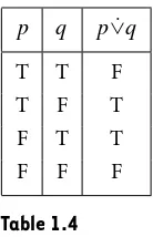
Given two statementspandq, we define the statementp∨q(porq) to be true precisely when at least one ofpandqis true, as illustrated in Table 1.3.This scenario illustrates why we consider p∨qto be true even when both pandq are true. We are just as happy if Megan is doubly covered by insurance rather than by one policy only. Because our conversational language is sometimes ambiguous when we use the word OR, we distinguish between two types of OR compound statements. We call∨theinclusiveOR. If you want to discuss an OR statement where you meanporqbut not both, use theexclusiveOR,p˙∨q. See Truth Table 1.4. Although we’ll not use this very often, it is a nice term to have. Just remember that use of the word OR in mathematical writing always means inclusive OR. For example, when we sayx y=0implies that either x=0ory=0, we include the possibility that bothxandyare zero.
p q p˙∨q
T T F
T F T
F T T
F F F
Table 1.4
Now we can build all kinds of compound statements.
Example 1.1.4.
Construct truth tables for the statements1. (p∧q)∨(¬p∧ ¬q), 2. p∧(q∨r),
3. (p∧q)∨(p∧r).
Solution:
See Table 1.5 for part 1 and Table 1.6 for parts 2 and 3 of Example 1.1.4. Some of the intermediate details are left to you in Exercise 1. Notice how we set up thep,q, andrcolumns for more than two given statements.p q ¬p ¬q p∧q ¬p∧ ¬q (p∧q)∨(¬p∧ ¬q)
T T F F T F T
T F F T F F F
F T T F F F F
F F T T F T T
p q r q∨r p∧(q∨r) p∧q p∧r (p∧q)∨(p∧r)
T T T T T T T T
T T F T T T F T
T F T T T T
T F F F F F
F T T F F
F T F F F
F F T F F
F F F F F
Table 1.6
Solutions to Example 1.1.4, parts 2 and 3
■
1.1.4 Logical equivalence
There are often several ways to say the same thing. We need to address the situation where two different constructs involving statements should be interpreted as having the same meaning, or as beinglogically equivalent. As a trivial example, consider thatp∧qshould certainly be viewed as having the same meaning asq∧ p. To build a truth table would produce identical columns forp∧qandq∧p. This is the way we define our use of the termlogical equivalence.
Definition 1.1.5.
Two statements are said to belogically equivalentif they have precisely the same truth table values. Ifpandqare logically equivalent, we writep⇔q.Look at parts 2 and 3 of Example 1.1.4. To illustrate the reasonableness of declaring p∧(q∨r)logically equivalent to(p∧q)∨(p∧r), consider the following criteria for being allowed to rent a car:
p: Megan has a valid driver’s license. q : Megan has her own insurance policy.
r: Megan bought the rental company’s insurance coverage.
Notice that saying “pAND eitherq orr” has the same meaning to us as “pandq, OR pandr.” This is a sort of distributive property; that is,∧distributes over∨, exactly like multiplication distributes over addition in real numbers. Exercise 5 asks you to demonstrate that∨also distributes over∧.
1.1.5 Tautologies and contradictions
she does not” would make you think, “Of course!” or “Naturally this is a true statement regardless of the circumstances.” A statement whose truth table values are all TRUE is called atautology. You’ll do the following in Exercise 6.
Example 1.1.6.
Show that¬(p∧q)∨(p∨q)is a tautology.A statement such as the one in Example 1.1.6 would be very confusing if expressed in English form. It would read something like,
Either it is not true that Dave has brown hair and green eyes, or he has either brown hair or green eyes.
One last item. The negation of a tautology is called acontradiction. The truth table values of a contradiction are all FALSE. In the same way that a tautology is the kind of statement that makes you think “Of course!,” a contradiction makes you think “No way can that ever be true!” A really easy example of a contradiction is p∧ ¬p. Sincepand
¬pcannot ever both be true,p∧ ¬pis always false. Tautologies and contradictions are very useful, as we will begin to see in Section 2.1.
E X E R C I S E S
1. Construct truth tables for the following statements: (a) p∨(q∨r)
(b) (p∨q)∨r (c) p∧(q∨r)
(d) (p∧q)∨(p∧r)
2. Which of the statements in Exercise 1 are logically equivalent?
3. Parts (a) and (b) of Exercise 1 show that∨ has the associative property. We can therefore allow ourselves the freedom to write p∨q∨rand understand it to mean either(p∨q)∨rorp∨(q∨r). Does∧have the associative property? Verify your answer with a truth table.
4. Below are several logical equivalences that are calledDeMorgan’s laws(a name you’ll want to remember). Verify these forms of DeMorgan’s laws with truth tables: (a) ¬(p∧q); ¬p∨ ¬q
(b) ¬(p∨q); ¬p∧ ¬q
(c) ¬(p∧q∧r); ¬p∨ ¬q∨ ¬r (d) ¬(p∨q∨r); ¬p∧ ¬q∧ ¬r
5. Show that∨distributes over∧.
6. Show that¬(p∧q)∨(p∨q)from Example 1.1.6 is a tautology.
8. Use DeMorgan’s laws from Exercise 4 as a basis for symbolic substitution and manip-ulation to show that¬[(p∨q)∧r]is logically equivalent to(¬p∧ ¬q)∨ ¬r by transforming the former statement into the latter. Use a similar technique to construct a statement that is logically equivalent to¬[p∨(q∧r)].
1.2 If-Then Statements
In this section, we want to do two things: 1) Consider the logical structure of the statement that p impliesornecessitatesq and its variations; and 2) return to the idea of logical equivalence and its connection to tautologies. We set the stage with a classic (albeit tired) example.
In my junior high school days, there was a man named Mr. Shephard who would stand in the middle of the street in front of my school every afternoon and flag down cars to try to get a ride to the post office. What made this dangerous stunt notable was the way Mr. Shephard often dressed. If there was even a single cloud in the sky, Mr. S would certainly be wearing his raincoat and carrying his umbrella. However, there were also days without a cloud in the sky on which Mr. S would be wearing his rain attire. When I think back about that period of my life, I am struck with the following fact: On every day that there were any clouds, Mr. S was undoubtedly dressed for rain. Granted, there might have been some clear days that he also dressed for rain, but I am not referring to this possibility in my claim. I’m only making an observation about something that happened on cloudy days.
1.2.1 If-then statements
From this little story, we want first to analyze the correlation between the weather and Mr. Shephard’s attire. Specifically, we want to define logically with a truth table what we mean by a statement such as “If it is a cloudy day,thenMr. S wears his rain gear.” In general, we consider the statement “Ifp, thenq,” which we write as p→q.
Let’s isolate one particular day, say day 1. Define statements p1 : Day 1 is a cloudy day.
q1 : Mr. S wears his rain gear on day 1.
Pretend for the moment that words like IF, THEN, and IMPLIES are not in your vocabulary. How can we piece together a logical statement using onlyp1,q1,∧,∨, and
¬that has the same sense asp1 →q1?3There are several possible answers. Here are two.
Read them as sentences to understand their meaning.
¬p1∨(p1∧q1) (1.1)
¬p1∨q1 (1.2)
Statements 1.1 and 1.2 are logically equivalent, but 1.2 is simpler, so let’s use it as our definition of p→q. We build its truth table:
Definition 1.2.1.
The statementp→q(read “Ifp, thenq” or “pimpliesq”) is defined to be a statement that is logically equivalent to¬p∨q, as illustrated in Table 1.7. We callpthehypothesis conditionandqtheconclusion.
p1 q1 ¬p1∨q1(⇔p1→q1)
T T T
T F F
F T T
F F T
Table 1.7
Notice from the definition that constructing a truth table for→produces FALSE only when the hypothesis condition is true and the conclusion is false.
Example 1.2.2.
Construct truth tables for the following statements.1. p→ ¬q 2. (p∧q)→r
Solution:
See Tables 1.8 and 1.9.p q ¬q p→ ¬q
T T F F
T F T T
F T F T
F F T T
Table 1.8
Solution to
Example 1.2.2, part 1
p q r p∧q (p∧q)→r
T T T T T
T T F T F
T F T F T
T F F F T
F T T F T
F T F F T
F F T F T
F F F F T
Table 1.9
Solution to Example 1.2.2,
part 2
1.2.2 Variations on
p
→
q
Given two statements p andq, we might want to analyze other possible correlations between their truth besidesp→q. Defining:
p: It is a cloudy day, q : Mr. S dresses for rain, we might address the following variations ofp→q.
q → p: If Mr. S dresses for rain, then it is a cloudy day. (Converse)
¬p → ¬q : If it is not a cloudy day, then Mr. S does not dress for rain. (Inverse)
¬q→ ¬p: If Mr. S does not dress for rain, then it is not a cloudy day. (Contrapositive)
Example 1.2.3.
Which, if any, of the statements p→q, q→p, ¬p→ ¬q, and¬q→ ¬pare logically equivalent?
Solution:
We construct a truth table (see Table 1.10).p q ¬p ¬q p→q q → p ¬p→ ¬q ¬q → ¬p
T T F F T T T T
T F F T F T T F
F T T F T F F T
F F T T T T T T
Table 1.10
Notice that the original statementp→qis logically equivalent to its contrapos-itive¬q → ¬p, and that the converseq→pis logically equivalent to the inverse
¬p→ ¬q. ■
There is one last construct involving if-then. Sometimes we want to consider the statement that we would call true precisely when pandq are either both true or both false. For example, if Mr. S had been firing on all cylinders we could have observed the following: Mr. S dressed for rain if it were cloudy, and if he dressed for rain, then it was a cloudy day. That is, he would have dressed for rainif and only if it were cloudy.
Definition 1.2.4.
Given statementspandq, the statementp↔q(read “pif and only ifHow can you use→,∧, and∨onpandqto construct a statement that is logically equivalent to p ↔q?4One answer is in the next example, and you’ll create others in
Exercise 2.
Example 1.2.5.
Show that(p→q)∧(q → p)is logically equivalent top↔q.Solution:
See Table 1.11.p q p↔q p→q q → p (p→q)∧(q → p)
T T T T T T
T F F F T F
F T F T F F
F F T T T T
Table 1.11
■
1.2.3 Logical equivalence and tautologies
In Section 1.1, we defined two statements to be logically equivalent if they have exactly the same truth table values. With the definition of p↔q, we can now offer an alternate definition of logical equivalence.
Definition 1.2.6.
Two statementspandqare logically equivalent if the statementp↔qis a tautology.
As we noted in Section 1.1.4, the significance of statements being logically equivalent is that they are different ways of saying precisely the same thing. Ifpis logically equivalent toq, then knowingpis true guarantees thatqis true, and vice versa.
If p↔qis a tautology, what does that say aboutp→qandq → pseparately?5If
p ↔qis a tautology, then p → qandq → pmust both be tautologies, too. Loosely speaking, the truth ofpis sufficiently strong to imply the truth ofqand vice versa. That is, in any case wherepis true, it can also be noted thatqwill, without exception, be true, and vice versa.
Example 1.2.7.
Show that p → q and¬q → ¬p are logically equivalent using Definition 1.2.6.Solution:
We already know that the truth table columns forp→qand¬q→ ¬p are identical, but we are asked to use Definition 1.2.6. Therefore, we construct4Take a hint from the sentence, “For example, if Mr. S had been firing on all cylinders . . . .” 5Rememberp
p q ¬p ¬q U V U →V V →U (U →V)∧(V →U)
T T F F T T T T T
T F F T F F T T T
F T T F T T T T T
F F T T T T T T T
Table 1.12
(p→q)↔(¬q→ ¬p) and show that it is a tautology. Writing p → q asU and¬q → ¬p as V, the details are displayed in Table 1.12. Since the last col-umn of Table 1.12 is a tautology,U andV are logically equivalent. Notice that the columnsU →V andV →Uare tautologies to make this last column a tautology.
■
Now let’s consider the situation where p↔qis not a tautology, but one ofp →q orq → pis. If p→qis a tautology whileq → pis not, then we say thatpis astronger statementthanq. This means that the truth ofpnecessitates the truth ofq, but the truth ofqis not necessarily accompanied by the truth of p.
Example 1.2.8.
Which statement is stronger,porp∧q? Verify with a truth table (see Table 1.13).p q p∧q (p∧q)→ p p→(p∧q)
T T T T T
T F F T F
F T F T T
F F F T T
Table 1.13
Solution:
Since(p∧q) → pis a tautology while p → (p∧q)is not, p∧q is stronger thanp. Knowingp∧q is true guarantees thatpis true, but knowing pistrue does not guarantee thatp∧qis true. ■
Example 1.2.9.
Which statement do you think is stronger,(p∧q)→ r or p → r? Determine for sure with a truth table.p q r p∧q U :(p∧q)→r V : p →r U→V V →U
T T T T T T T T
T T F T F F T T
T F T F T T T T
T F F F T F F T
F T T F T T T T
F T F F T T T T
F F T F T T T T
F F F F T T T T
Table 1.14
■
Notice this important fact. StatementsUandV from Example 1.2.9 have the same conclusion, but the hypothesis condition forU(p∧q) is stronger than the hypothesis condition forV (p). However,U is a weaker statement thanV. Exercise 4 asks you to investigate and explain from the truth table why an if-then statement is weakened when the hypothesis condition is strengthened.
What is the significance of one statement being stronger than another? Here is an example. Define the following statements:
p: Megan is at least 25 years old. q : Megan has a valid driver’s license. r : Megan is allowed to rent a car.
What does it mean to say thatV(p→r) is stronger thanU((p∧q)→r)?6StatementU
says that age and a license will guarantee your eligibility to rent a car. StatementV says that age alone is sufficient to be eligible. Thus, if everyone at least 25 years old can rent a car, then certainly everyone at least 25 with a license can, too. Thus if V is true, so isU. On the other hand, just because licensed people at least 25 years old can rent a car, it does not follow that all people over 25 can do the same. That is,U does not implyV.
Example 1.2.10.
Without justifying by proof, state whether the following statements are logically equivalent, whether one is stronger than the other, or neither.1. p: xis an integer that is divisible by 6.
q : xis an integer that is divisible by 3.
2. p: x3−4x2+4x=0
q : x∈ {0,2,4}